| home |
| theory |
| apparatus |
| procedure |
| data |
| bibliography |
| contact |
Experiment: Titration of mica
The goal of this procedure is to demonstrate titration of the surface charge of mica. The result will be a graph showing the dependence of zeta potential on pH in a background of aqueous KCl. For details of the interaction of mica with aqueous solutions, see the background discussion in the data pages in the menu at left.
1. Find the sample support cylinder with the mica disk attached. Cleave the mica by applying clear packaging tape to the entire surface of the sample. Apply the tape and rub the taped surface against a flat surface (or using a gloved finger) to remove air bubbles. Once the tape is as flush as possible with the mica, slowly pull the tape upward from one side. Observe the detachment of a layer of mica. A good cleave leaves the remaining surface smooth and mirror-like and leaves a very thin layer of mica on the tape. It may be necessary to cleave again if the surface is flaky and visibly defective. Place the cleaved sample up to a few mm above the plane of the sample in a solution of pH=11 for 30 minutes prior to testing.
2.While the sample is equilibrating with the pH 11 solution, calibrate the pH and conductivity probes. The pH probe is calibrated with standard solutions at pH of approximately 4, 7, and 10. Calibrate the conductivity meter with a solution of 100 microSieman/cm solution, or make your own calibration solutions with a value in this vicinity. Make sure to account for temperature and its affect on conductivity. It is very important to calibrate the conductivity meter accurately! All conversions of zeta streaming potential to zeta potential require multiplication by the conductivity, so error in conductivity translates directly to error in zeta.
3. Make 100mL each of both 0.05 M acid (pH=2.2) and base (pH=11.8) for titrations.
4. Rinse the cell out with DI water and fill to the baffle line. Be careful not to damage the electrodes. Sonicate the cell for 15 minutes. Rinse again after sonication and fill to the baffle line. Place the cell in the ZetaSpin mount and twist it to secure its location. Make sure the lid is flush with the Teflon cell. Attach the conical centering piece to the spindle. Raise the cell so that the centering piece is close to the center electrode. Use the micrometer adjustments to center the tip over the reference electrode pointing upward along the cell’s axis.
5. Lower the cell and remove the centering piece. Remove the cylinder bearing the sample from the pH 11 bath and thread it snugly on to the spindle. Insert the pH and conductivity probes. Attach the red wire of the nanovoltmeter to the center electrode and the black wire to the other electrode. Raise the cell until the electrode is just below the sample. A reflection of the electrode can be seen from below on the surface of the sample using a backlight. When the electrode and its reflection almost meet, the electrode is just below the sample. Lower the cell one full rotation of the vertical translation stage, which is 1 mm.
6. Use the toggle switch on the MSRX speed control box to power up the motor. Manually set the sample rotation at 2000 rpm by punching the far left button on the MSRX. Add a sufficient volume of 10,000 µS/cm KCl solution (about 3-4 mL) to make a solution with a conductivity of 150 µS/cm. Periodically “jiggle” the conductivity probe to remove any gas bubbles that have accumulated inside the probe. Check the pH; it should be between 5 and 6. If the pH is less than 5 or more than 8, then lower the cell, empty it, and start over at the point where you add DI water to the cell. If the pH is between these limits, correct it to 5.5 < pH < 6. This concludes the setup phase.
IMPORTANT: RESET THE MSRX MOTOR CONTROLLER TO ZERO ROTATION BEFORE ACTIVATING COMPUTER CONTROL. DO IT NOW.
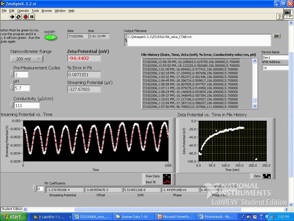
7. Turn on the computer and click on the ZetaSpin icon to load the Labview interface. The ZetaSpin operates in two modes, single shot and continuous. To make a single shot measurement, click the on/off button to make it green. Then click the white arrow in the upper left corner of the screen immediately under Edit. The spindle speeds up and slows down approximately 10 times, after which fresh data appear on the “Streaming Potential vs time” graph in the middle of the screen toward the left. The amplitude of the streaming potential during the modulation is reported in its box in the middle of the screen. The zeta potential is reported in red in the box in the upper middle of the screen. The pH, conductivity, and zeta potential are also reported in the table in the upper right corner. After this all happens, the motor stops and the ZetaSpin awaits further input. The advantage of the single-shot mode is that one can update the conductivity and pH for every measurement.
To make a continuous measurement, click on the button between the single-arrow button and the Stop sign in the upper left of the screen. The ZetaSpin now runs automatically, reporting data approximately every minute until stopped. To stop the sequence, wait until the motor is at a low speed point in any cycle, and click on the Stop sign. In continuous mode, the apparatus runs automatically, but the zeta potential might drift because the conductivity in the cell drifts while the input data remain the same; thus it is important to check the conductivity periodically.
8. Enter the conductivity and the pH in their respective boxes on the Labview Interface (LI). Click the on/off button to make the indicator green and then click the “Continuous” button at the top off the screen to begin making zeta potential determinations approximately once per minute. The computer is telling the nanovoltmeter to acquire streaming potential data and then display it on the graph to the left of the LI. Observe the streaming potential data and the fit between the data and the theory. The fit, as described in the theory section, should be almost perfect as in the screenshot presented on this website. The fitting process produces the value of the zeta potential, which should be in the vicinity of -80 mV. It sometimes happens that the data are ugly because of a malfunction of the reference electrodes. Sometimes the data look good, but the fit is offset such that the reported zeta is positive. In either case, call the Lab Instructor over to take a look if this is the case.
9. Let the cell operate for a few minutes. When the value of the zeta potential changes by less than 2 mV per measurement, stop the measurement and re-check the conductivity. Make 5 single-shot measurements, noting the conductivity and pH each time.
10. Change the pH by 1/2 a pH unit and repeat the above steps until you reach a pH of 9.5.
11. Lower the cell and empty it. Repeat the above process to prepare the apparatus for measurement. You do not have to re-soak the mica sample, however. Use the same sample surface. Now titrate down from pH 5.8 in increments of 1/2 pH units until the conductivity reaches 200 µS/cm and then titrate back up until the conductivity reaches 200 µS/cm. (The conductivity decreases as you first add base to an acidic solution and then increases as you add more. Why?)
12. Average the measured zeta potentials at each pH. Determine the 95% confidence intervals from the data at each pH. Plot the data with the confidence intervals as a function of pH. On the same graph, plot the following data taken from Scales et al. who carefully measured the zeta potential of mica in KCl using a version of the classical parallel plate apparatus.
pH |
zeta |
3.71 |
-32.4 |
3.95 |
-36.0 |
4.01 |
-43.9 |
4.35 |
-42.2 |
4.40 |
-54.7 |
4.57 |
-47.6 |
4.83 |
-54.4 |
5.08 |
-65.7 |
5.15 |
-59.8 |
5.47 |
-67.9 |
5.75 |
-76.3 |
5.94 |
-74.8 |
6.24 |
-77.2 |
7.52 |
-83.4 |
8.92 |
-83.6 |
9.80 |
-81.9 |
Table 1. Zeta potential of mica in contact with a 1 mM concentration of KCl. Taken from the following source: Peter J. Scales, Franz Grieser, and Thomas W. Healy “Electrokinetics of the Muscovite Mica-Aqueous Solution Interface,” Langmuir 1990, 6, 582-589.