DCGAN
Discriminator
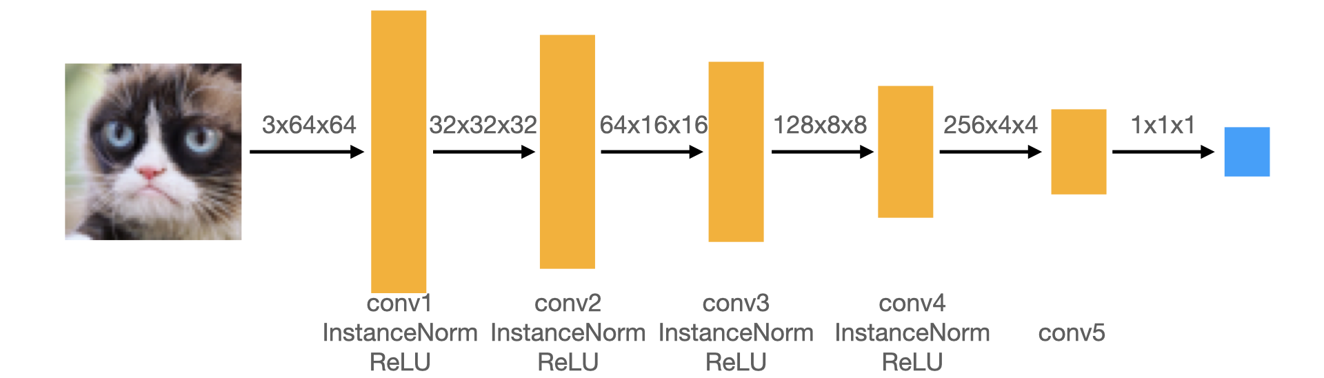
Discriminator Structure of DCGAN
In each convolutional layer, we reduce the spatial dimension of the input volume by a factor of 2. Given a kernel size (K) of 4 and a stride (S) of 2, the size of the padding can be calculated as follows:
$$ I_{new}=\frac{I_{old}+2P - K}{S} + 1 = \frac{I_{old} + 2P - 4}{2} + 1 = \frac{I_{old}}{2}+P-1 $$ $$ P=\frac{2I_{new}-I_{old}}{2}+1 $$
- Input to Conv1 to ... to Conv4: $$I_{old}=2I_{new} \quad \Rightarrow \quad P=1$$
- Conv4 to Conv5: $$I_{old}=4, I_{new}=1 \quad \Rightarrow \quad P=0$$
Generator

Discriminator Structure of DCGAN
The generator is essentially the inverse of the Discriminator. Notably, for the first layer (up_conv1), applying a convolution layer directly without any upsampling is advised to achieve a 4x4 output, as mentioned in the writeup.
The relationship between stride, padding, and kernel size is as follows:
- Noise to Conv1: $$I_{new}=\frac{I_{old}+2P - K}{S} + 1$$ $$3S=1+2P - K$$ $$2=2P - K$$
- Conv1 to up_Conv2: $$I_{new}=\frac{I_{old}+2P - K}{S} + 1$$ With an upscale layer, $I_{old} = I_{new}$. We select stride = 1, padding = 1, and kernel size = 3.
Loss
The loss implemented for the vanilla GAN is an improved version from the Least Squares Generative Adversarial Networks (LSGAN), offering greater stability than the sigmoid cross-entropy loss used in the original GAN paper.
The L2 Loss can be expressed as: $$\begin{aligned} \min _D V_{\mathrm{LSGAN}}(D) & =\frac{1}{2} \mathbb{E}_{\boldsymbol{x} \sim p_{\mathrm{data}}(\boldsymbol{x})}\left[(D(\boldsymbol{x} \mid \Phi(\boldsymbol{y}))-1)^2\right]+\frac{1}{2} \mathbb{E}_{\boldsymbol{z} \sim p_{\boldsymbol{z}}(\boldsymbol{z})}\left[(D(G(\boldsymbol{z}) \mid \Phi(\boldsymbol{y})))^2\right] \\ \min _G V_{\mathrm{LSGAN}}(G) & =\frac{1}{2} \mathbb{E}_{\boldsymbol{z} \sim p_{\boldsymbol{z}}(\boldsymbol{z})}\left[(D(G(\boldsymbol{z}) \mid \Phi(\boldsymbol{y}))-1)^2\right] \end{aligned}$$
Differentiable Augmentation
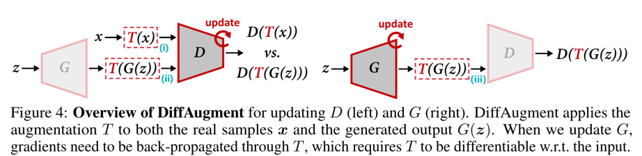
Differentiable Augmentation illustrated
Differentiable Augmentation, which allows gradients to pass through it, dynamically adds augmentation to both the generator and discriminator. This technique proves invaluable for guiding training in scenarios like ours, as GANs can easily overfit to small datasets, as demonstrated in my results below:
Experiment Results
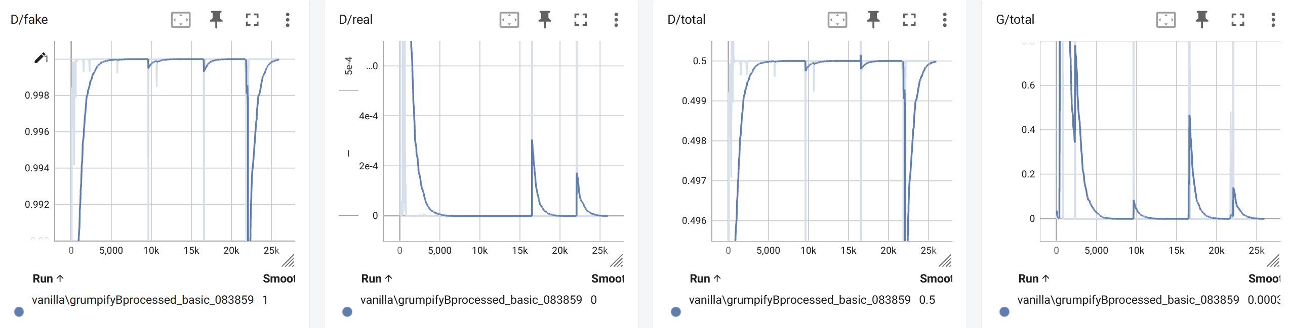
Basic data preprocessing + without differentiable augmentation
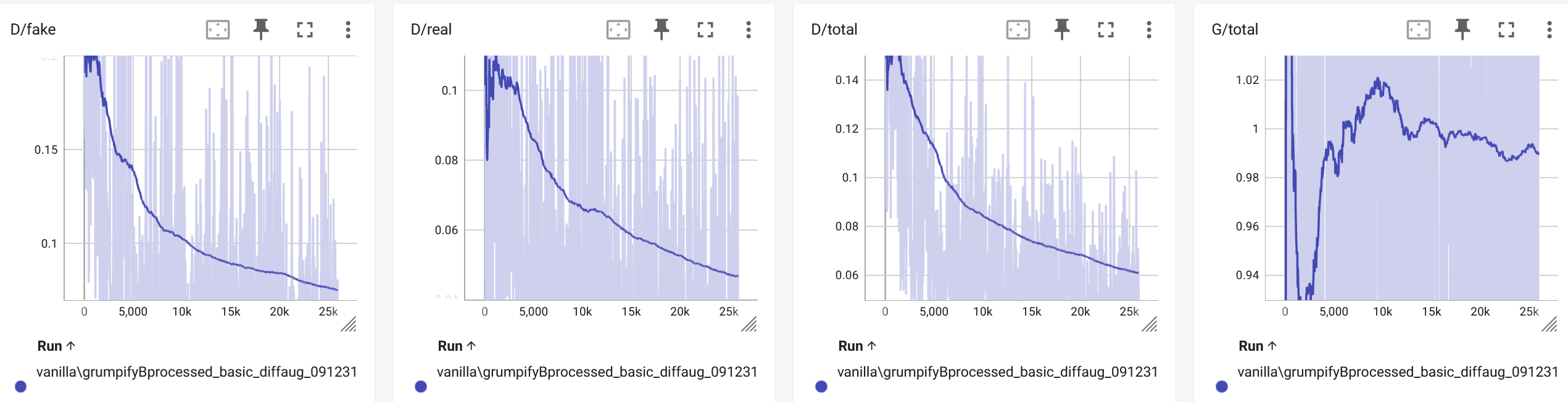
Basic data preprocessing + with differentiable augmentation
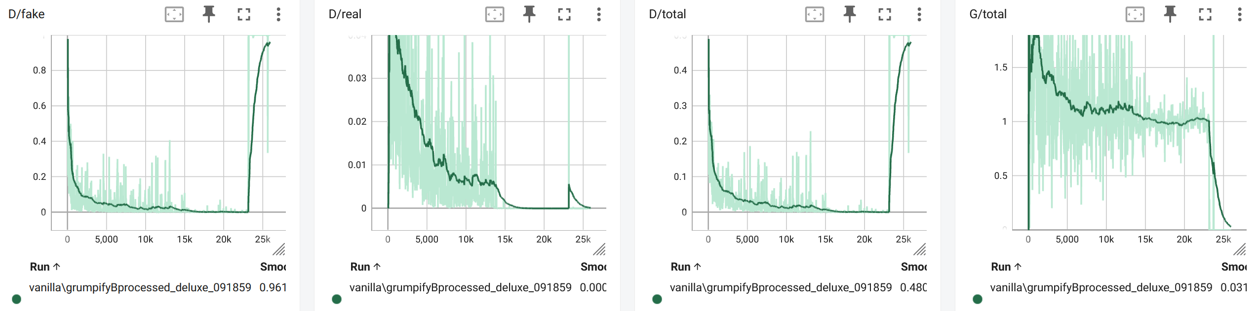
Deluxe data preprocessing + without differentiable augmentation
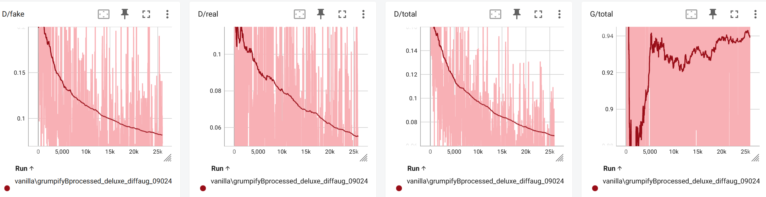
Deluxe data preprocessing + with differentiable augmentation
Observations
The most basic version quickly overfits, with discriminator loss remaining at 1 and generator loss at 0 most of the time. In other configurations, both discriminator and generator losses decrease gradually, indicating successful GAN training. However, training is more unstable without differentiable augmentation.
Samples Comparison
With `--data_preprocess=deluxe` and differentiable augmentation enabled, early training samples (e.g., iteration 200) show only a blurry blob, while later samples are much more detailed, with clear cat eyes and more distinct facial features. The images become sharper, with fewer glitch-like artifacts as training progresses.
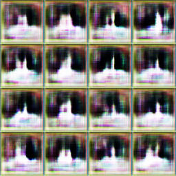
Samples at iteration 200
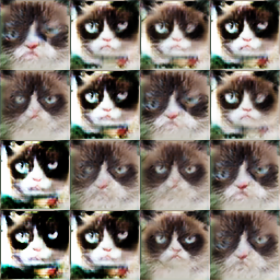
Samples at iteration 25800
Normalization Method Importance
Experimentation revealed that the normalization method in convolutional layers significantly impacts training, with instance normalization yielding the best performance.
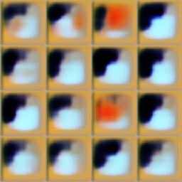
Model fails to converge with `norm=None`
CycleGAN
The structure of the CycleGAN Generator closely resembles that of the DCGAN Discriminator, with the addition of ResBlocks and a reversal akin to the DCGAN Generator, as illustrated below:
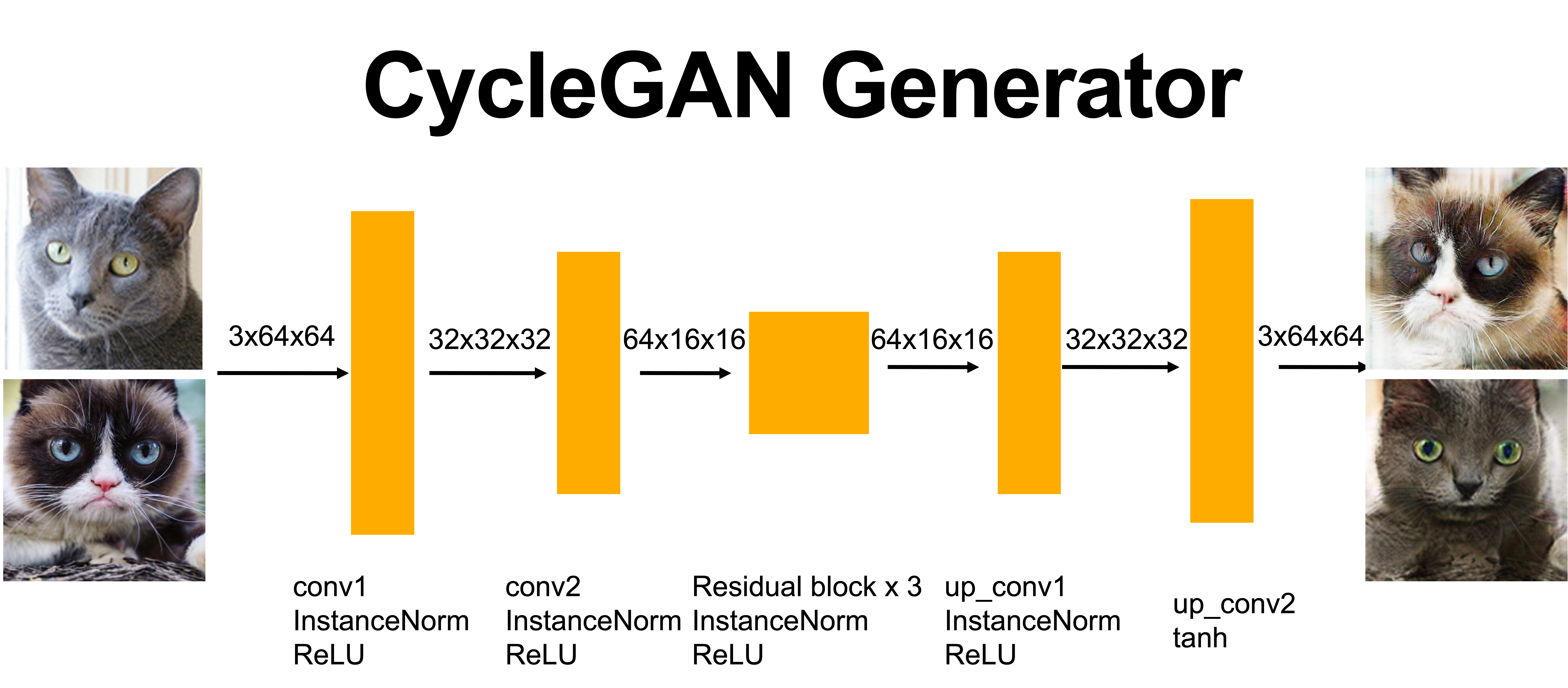
Structure of CycleGAN
CycleGAN also employs a PatchDiscriminator, outputting results as a grid (patches). This can be achieved by replacing the last convolutional layer in the DCGAN discriminator with a flattening layer.
CycleGAN Loss
I regard CycleGAN's loss as a symmetric version of DCGAN's, encompassing loss from domain X to Y and vice versa. Differentiable augmentation can also be applied to CycleGAN, with implementation nearly identical.
Discriminator Loss
$$\mathcal{J}_{\text {real }}^{(D)}=\frac{1}{m} \sum_{i=1}^m\left(D_X\left(x^{(i)}\right)-1\right)^2+\frac{1}{n} \sum_{j=1}^n\left(D_Y\left(y^{(j)}-1\right)^2\right.$$ $$\mathcal{J}_{\text {fake }}^{(D)}=\frac{1}{m} \sum_{i=1}^m\left(D_Y\left(G_{X \rightarrow Y}\left(x^{(i)}\right)\right)\right)^2+\frac{1}{n} \sum_{j=1}^n\left(D_X\left(G_{Y \rightarrow X}\left(y^{(j)}\right)\right)\right)^2$$
Cycle Consistency Loss in Generator Loss
The intuitive idea that an image transformed from domain X to Y and then back to X should remain unchanged forms the basis of the cycle consistency loss in CycleGAN. This loss, the L1 or L2 norm between the source image y^{(i)} and the reconstructed image $G_{X \rightarrow Y}\left(G_{Y \rightarrow X}\left(y^{(i)}\right)\right)$, ensures transformations between domains X and Y do not alter the core structure.
The final loss for the generator includes both the transformation and cycle consistency components, emphasizing the reversible nature of the transformations between domains.
Experiment Results
1000 iterations, w/ and w/o cycle-consistency loss

w/o cycle consistency, X-Y
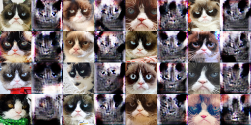
w/o cycle consistency, Y-X
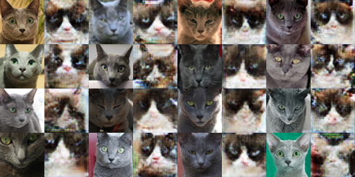
w/ cycle consistency, X-Y
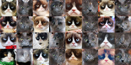
w/ cycle consistency, Y-X
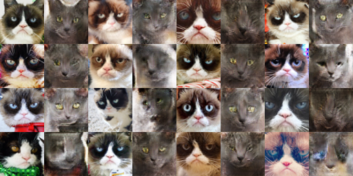
10000 iterations, w/ and w/o cycle-consistency loss, cat dataset
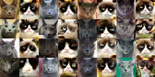
w/o cycle consistency, X-Y
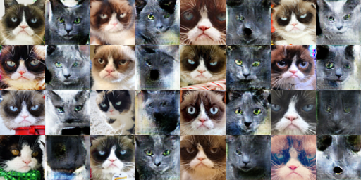
w/o cycle consistency, Y-X
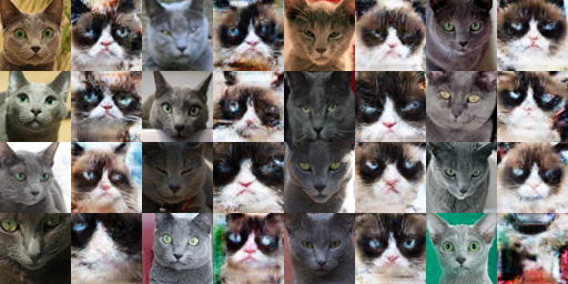
w/ cycle consistency, X-Y
w/ cycle consistency, Y-X
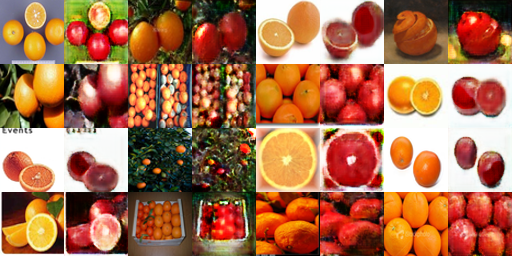
10000 iterations, w/ and w/o cycle-consistency loss, apple-orange dataset
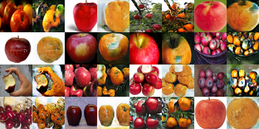
w/o cycle consistency, X-Y
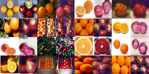
w/o cycle consistency, Y-X
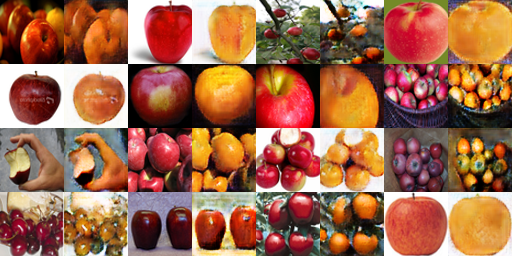
w/ cycle consistency, X-Y
w/ cycle consistency, Y-X
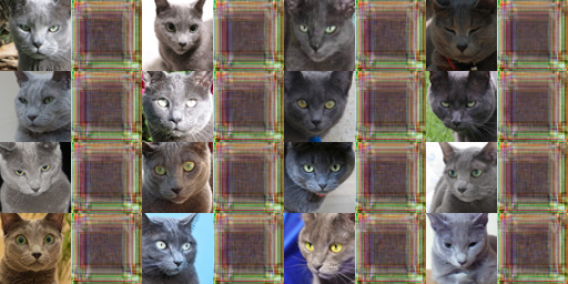
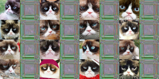
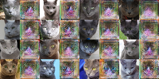
10000 iterations, w/ and w/o cycle-consistency loss, cat dataset, DCDiscriminator
w/o cycle consistency, X-Y, dc
w/o cycle consistency, Y-X, dc
w/ cycle consistency, X-Y, dc
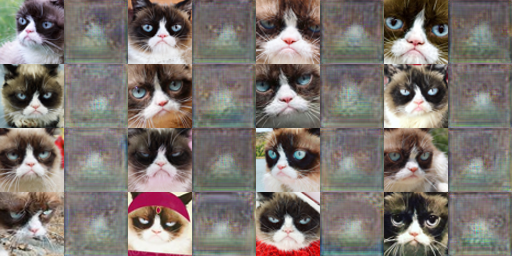
w/ cycle consistency, Y-X, dc
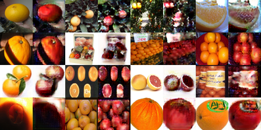
10000 iterations, w/ and w/o cycle-consistency loss, apple-orange dataset, DCDiscriminator
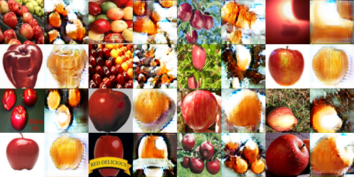
w/o cycle consistency, X-Y, dc
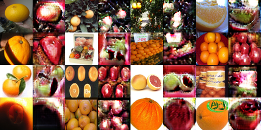
w/o cycle consistency, Y-X, dc
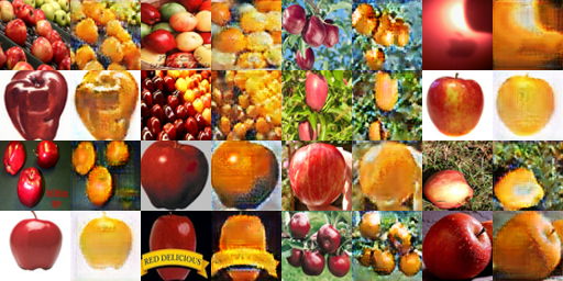
w/ cycle consistency, X-Y, dc
w/ cycle consistency, Y-X, dc
Observations
Regarding cycle consistency, it is evident that models trained with cycle consistency loss retain more original features, such as the stem of an apple when it is transformed into an orange. This demonstrates the effectiveness of cycle consistency in preserving original features, leading to results that closely resemble the original image. Conversely, models lacking cycle consistency loss tend to produce more artifacts and generate images less similar to the original, underlining the importance of cycle consistency in maintaining original attributes. While this generally enhances image quality, it may also inadvertently preserve undesired features, like an apple's stem on an orange.
The use of a DCDiscriminator results in inferior outcomes compared to employing a PatchDiscriminator, particularly noticeable in cat image datasets. Models with a DCDiscriminator generate vague, indistinct shapes, whereas those with a PatchDiscriminator produce sharper, more detailed images. This difference aligns with the theoretical understanding that PatchDiscriminators are capable of discerning finer local details, whereas DCDiscriminators tend to capture more generalized global information.
Improvements
Diffusion Model
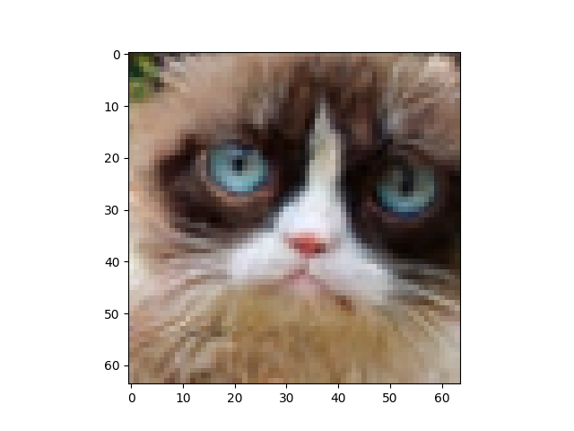
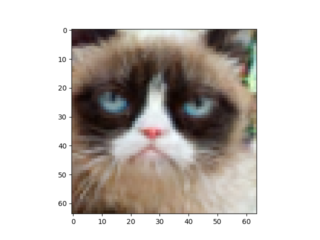
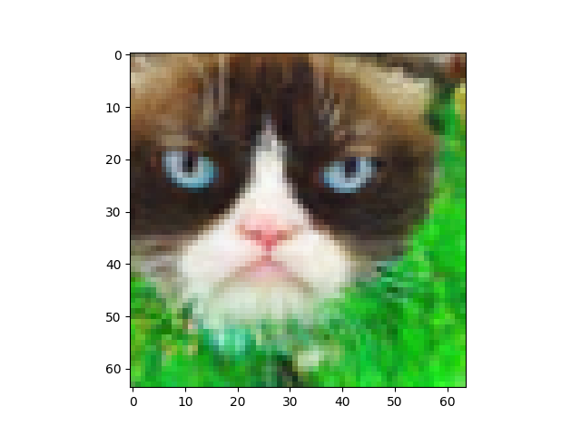
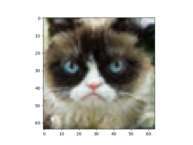
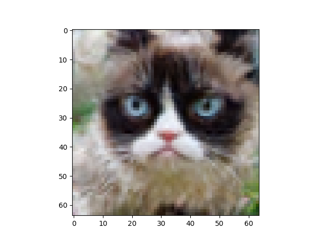
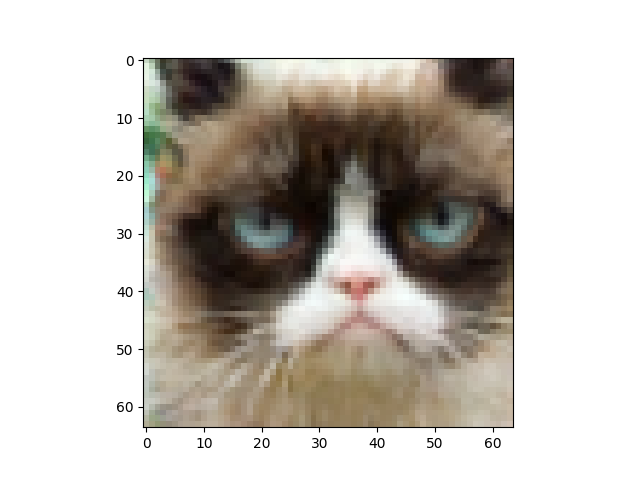
Following the template, I implemented a diffusion model. The results were surprisingly good, surpassing those of the GAN, although achieving them took longer.
Loss Improvement: WGAN
The traditional GAN framework seeks to minimize the KL divergence between the real and generated data distributions. However, an alternative approach involves using a different metric for this purpose. Inspired by Optimal Transport theory, the Earth Mover (EM) distance offers a novel perspective:
$$W\left(P_r, P_g\right)=\inf _{\gamma \in \Pi\left(P_r, P_g\right)} \mathbb{E}_{(x, y) \sim \gamma}[\|x-y\|]$$
This metric conceptualizes the task as minimizing the "cost" needed to transform the generated data distribution into the real data distribution. According to the Kantorovich-Rubinstein Duality, the Earth Mover distance can be reformulated as:
$$W\left(P_r, P_g\right)=\sup _{\left\|f_L\right\| \leq 1} \mathbb{E}_{x \sim P_r}[f(x)]-\mathbb{E}_{x \sim P_g}[f(x)]$$
In the context of WGAN, this duality leads to a loss function aiming to minimize the Wasserstein distance. The formulation of this objective includes not only the direct comparison of distributions but also a term enforcing the Lipschitz constraint, essential for the model's stability:
$$\begin{gathered} \max _D \underbrace{\mathbb{E}_{x \sim P_r}[D(x)]-\mathbb{E}_{\tilde{x} \sim P_g}[D(\tilde{x})]}_{\text {Wasserstein critic objective }}+\lambda \underbrace{\mathbb{E}_{\hat{x} \sim P_{\hat{x}}}\left[\left(\left\|\nabla_{\hat{x}} D(\hat{x})\right\|_2-1\right)^2\right]}_{\text {Gradient Penalty for Lipschitzness }} \\ \hat{x} \leftarrow \epsilon x+(1-\epsilon) \tilde{x} \end{gathered}$$
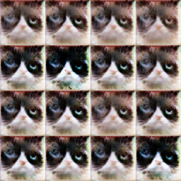
Here, $\hat{x}$ represents a blend between real and generated samples, facilitating the gradient penalty's application and ensuring the discriminator's smoothness. This nuanced approach to defining the loss function underpins the WGAN's improved stability and performance over its predecessor.
WGAN Generated Sample