Neural Style Transfer
1. Introduction
In this assignment, a neural style transfer which resembles specific content in a certain artistic style will be implemented. The algorithm takes in a content image, a style image and output a stylized image which matches the content input in content distance space and the style input in style distance space by optimizing either a random input or a copy of content image.
In part 1, the content loss will be implemented to optimize a random noise in content space to a given content image. The ablation study is conducted on which layer of the encoder network to be used, and different noise is drawn to demonstrate the stability of the algorithm.
In part 2, the style loss will be implemented by using Gram matrix as a style measurement to optimize a random noise in style space to a given style image. The ablation study is conducted on which layer of the encoder network to be used, and different noise is drawn to demonstrate the stability of the algorithm.
In part 3, we combine the content loss and style loss to perform neural style transfer by optimizing either a random input or a copy of content image to match the content input in content distance space and the style input in style distance space.
I also 1) run style transfer on grump cats from the previous homework; 2) apply style transfer to a video (frame by frame); 3) add histogram loss to make results more stable; 4) implement a feedforward network to output style transfer results directly for Bells & Whistles. The results is also shown in part 3.
2. Content Reconstruction
Denote the Lth-layer feature of input image X as \(f_L^X\) and that of target content image as \(f_L^C\). The content loss in this assignment is defined as the sum of squared L2-distance of selected features \(\mathcal{L_{content}}=\sum_{l\in \Gamma}|f_l^X - f_l^C|^2_2\), where \(\Gamma\) is the set of layers of the model used to extract the content features. In this assignment, the first layer of the each convolution block of VGG19 is used to extract the features, and each is named as \(conv\_1, ..., conv\_5\).
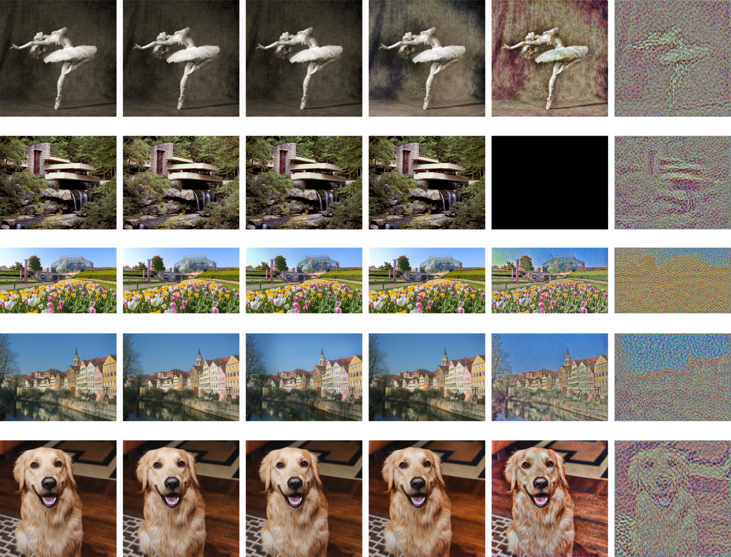
Result
I apply the content reconstruction for all five content images using two different noise inputs, and the result is ablated on using different convolution blocks of VGG19. The loss saved by tensorboard can be checked here. The final results are shown as below.
-
Content Reconstruction Result. Each Row (from top to bottom): dancing, fallingwater, phipps, tubingen, wally. Each Column (from left to right): original, conv_1, conv_2, conv_3, conv_4, conv_5
Note that the gradients explode for fallingwater using conv_4 due to some unknown reasons (even for both input noise), so the results are black. And for phipps using conv_2 with SEED=27, the result looks wired (like the sky is green), but if we check the loss, actually it has the lower loss value than the "normal" case reconstructed using conv_2 with SEED=13. It demonstrates that the network actually regard the output result is more similar to the reconstructed image in the feature space. Have no idea why but maybe just a wired initialization make the algorithm break.
Discussion
Basically, as the layer used to extract content features goes deeper, we can see the reconstructed content images are worse. One reason is that as the network goes deeper, more gradients accumulate and it will be harder for the optimizer to optimize the input image based on these gradients. This is proved by the extremely high losses when we use the conv_4 and conv_5 reconstructed content images. Also, generally we will say the deeper layer of a convolutional network will tend to capture higher-level information and representation of the input image, so that even two images look different by human being, they can still have the similar high-level representation for a neural network, making it not reasonable to use deep layer of a network to reconstruct image content.
3. Texture Synthesis
Denote the Lth-layer feature of input image X as \(f_L^X\) and that of target style image as \(f_L^C\). Both features are of shape \((B, C, H, W)\) (\(B=1\) in this assignment as we just optimize one image each time). To compute the style loss, we first reshape the feature to \((B\times C, H\times W)\), and then compute the gram matrix normalized over feature pixels by \(G=\frac{f f^T}{B\times C\times H\times W}\). And the style loss will be \(\mathcal{L_{style}} = \frac{\sum_{l\in \Upsilon}|f_l^X (f_l^X)^T - f_l^C (f_l^C)^T|^2_2}{B\times C\times H\times W}\), where \(\Upsilon\) is the set of layers of the model used to extract the style features.
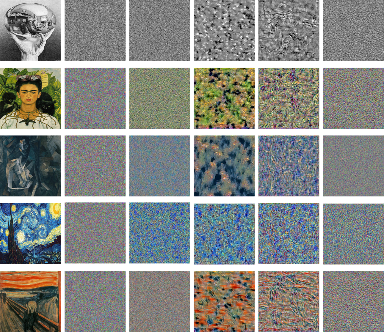
Result
I apply the texture synthesis for all five style images using two different noise inputs, and the result is ablated on using different convolution blocks of VGG19. The loss saved by tensorboard can be checked here. The final results are shown as below.
-
Texture Synthesis Result. Each Row (from top to bottom): escher_sphere, frida_kahlo, picasso, starry_night, the_scream. Each Column (from left to right): original, conv_1, conv_2, conv_3, conv_4, conv_5
Discussion
As opposed to the content reconstruction case, in the texture synthesis, we generally want a higher-level information and representation of the input image so that the synthesized texture will focus more on the global structure, color and style of the input image instead some low-level local details. We can see from the figure above that, basically as the layer used to extract style features goes deeper, the synthesized texture becomes better. Specifically, for using conv_1 and conv_2 as the input layer, the synthesized textures are kind of noises which capture the similar color of the input style image. While for using conv_3 and conv_4 as the input layer, the synthesized textures can follow the characteristics and patterns which exist in the original style input. But the results get worse when we use conv_5, as it is too deep so that make it difficult for the optimizer to optimize based on these gradients.
4. Style Transfer
The implementation of gram matrix and style loss is elaborated in part 3. The layer conv_2 is chosen to extract the features for content loss as it won't be too deep to present the low-level information and structure of the content image, and won't be too close to input layer (like conv_1) so that it have enough gradients to back-propagate. The layer conv_3 is chosen to extract features for style loss as it's deep enough to present some high-level information of the style image while won't be too deep for the optimizer to optimize.
I use the default hyperparameter as given in (\(\lambda_{content}=1, \lambda_{style}=1000000\))
to train the model for 300 epochs for using content image as initialization. And for
experiments with using random noise as input, I train the model for 1000 epochs with
\(\lambda_{style}\) 10 times smaller.
Following the section 4.3 of the paper, I implement the histogram loss to addresses
instabilities by ensuring that the full statistical distribution of the features is preserved.
Denote the Lth-layer feature of input image X as \(f_L^X\) and that of target style image as
\(f_L^C\), we first apply the histogram matching to the Two
features so that the cumulative distribution function (CDF) of values in each band of the input
feature matches the CDF of bands in target feature. And the histogram loss is the Frobenius norm
distance between the original feartures and the remapped ones. Formally, we calculate the remapped features by \[f{'}_L^{X} = hist\_rematch(f_L^X, f_L^C)\] And the histogram loss is \[\mathcal{L_{hist}}=\sum_{l\in \Theta}|f_l^X - f{'}_l^X|^2_{Fro}\],
where \(\Theta\) is the set of layers of the model used to extract the histogram features. I use
conv_3 in this assignment. Following the paper, I also implement a feedforward network to output
style transfer results directly in a single pass. The generator network is
exactly the same as the CycleGan generator I used Assignment 3 to generate high-resolution
output. The network is trained with the same style loss and content loss aforementioned, plus
the total variation loss to encourage spatial smoothness in the
output image. The style transfer network is trained on the MS-COCO dataset with input size of
\(128 \times 128\) and batch size of 32 to accelerate the training.
The network can converge with roughly one epoch over the training data. I used Adam with
learning rate \(1 \times 10^{-4}\) for optimization. Check my codes for more details.
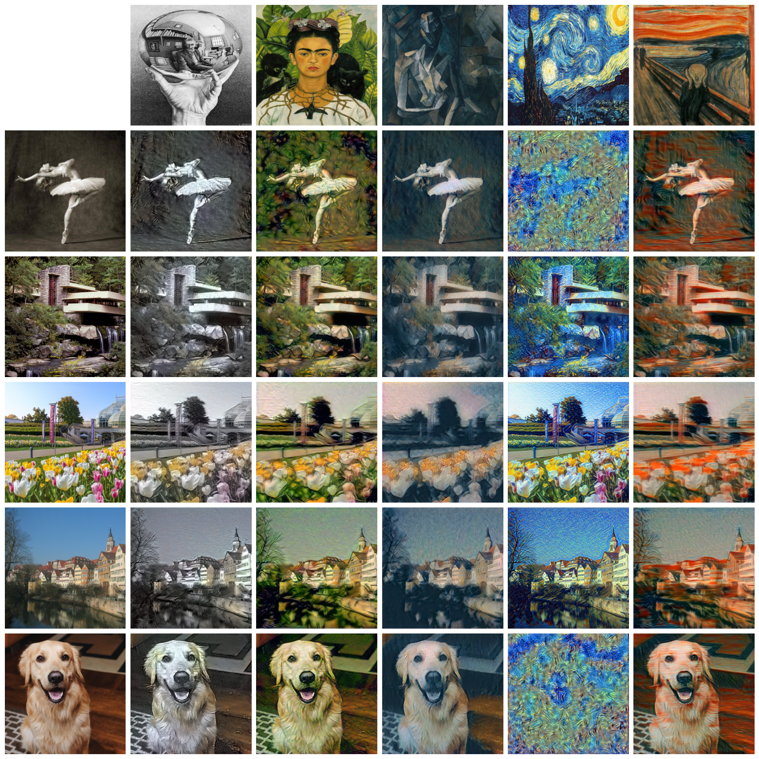
I apply the style transfer among all five style images and five content images with simple
setting using both content and noise initialization. Also, I test the histogram loss
using content initialization, and I also generate the results using the trained style network
for all content images. It's noted that although the feedforward network is trained on low resolution \(128 \times 128\)
images, it can still be tested on high resolution images, and the results shown below is inferenced with \(512 \times 512\) resolution. The final results are shown as below.
From the figure above, we can the using the content image as initialization preserve the content
input better, which is of course as the optimizer won't
bother to reconstruct the content information during optimization. While using random noise as
initialization sometimes can't reconstruct the
content well, for example the cases phipps+starry_night and wally+the_scream, the results using
random noise as initialization actually are more "stylized" and
can fuse the style and content information better as far as I concerned. The reason may be,
rather than just optimize the style from a given content image, optimizing the content
and style at the same time from a random initialization will help the network to combine and
fuse both the information from content and style input.
In terms of running time, using random noise as initialization is significantly slower to
converge than using the content image as initialization, and that's why
I run 1000 epochs for all the random initialization experiments.
The histogram loss addresses instabilities by ensuring that the full statistical distribution of
the features is preserved. As shown in the figure, the color space of the input image is more
like the style
images.
The feedforward network can output style transfer results directly in a single pass. But
different networks is needed to be trained for different styles. In my implementation,
the network can be trained with 25 minutes using a single NVIDIA GeForce RTX 2080 Ti GPU, and
the inferencing speed can be more than 40 FPS. Also the feedforward network somehow better
transfer the style in my opinion.
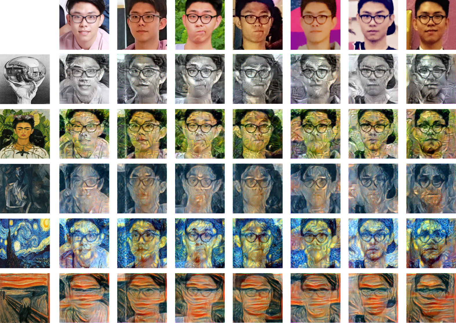
I create a Leo Dataset is last assignment which consists of my own faces from my
albums. And I run
the style transfer on some of these faces with provided style images. The result is shown below.
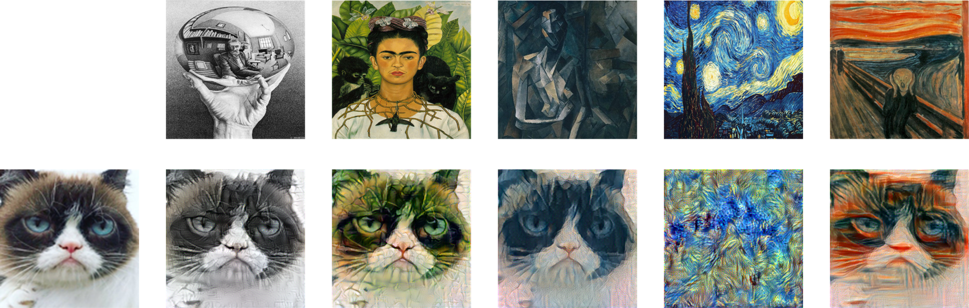
I run the style transfer on one of grump cat image with provided style images. The result is
shown below. I also try to run the style transfer on official music video for “No Love
(Extended Version)” where Summer Walker has dropped a remix of
her sultry single “No Love” with an assist from Cardi B. Note that the style transfer is
done by the feedforward network to highly speed up inferencing.
4.1 Histogram Loss
4.2 Feedforward Network
4.3 Result on Given Images
Style Transfer Result. Each Row (from top to bottom): style image, dancing,
fallingwater,
phipps, tubingen, wally. Each Column (from left to right): content image,
escher_sphere, frida_kahlo,
picasso, starry_night, the_scream.
4.4 Discussion
Content and Noise Initialization
Histogram Loss
Feedforward Network
4.5 More Result: Leo Dataset
Style Transfer Result on Leo Dataset. Each Row (from top to bottom): face image,
escher_sphere, frida_kahlo,
picasso, starry_night, the_scream.
4.6 More Result: Grump Cat
Style Transfer Result on Grump Cat. Each Column (from left to right): cat image,
escher_sphere, frida_kahlo,
picasso, starry_night, the_scream.
4.7 More Result: “No Love (Extended Version)” + Feedforward Network
Turn on the speaker and enjoy the song :D