Toy Problem

Poisson Blending formulates the blending objective function as a least squares problem where we want to find new instensity values "v" given the source region "S", the source image "s", and the target image "t".

However, this is a lot to tackle at once, so we will start with a simpler problem. We will extract all of the x and y gradients from a simple rgb image and use a single pixel value to reconstruct the image. Our least squares conditions become to minimize

After implementing the least squares objective, we solve using scipy.sparse.linalg.lsqr and the reconstructed image is the same as the original.

Poisson Blending

Now that we have the infastructure, we can tackle Poisson Blending. This requires finding "v" that minimizes

This works by iterating through each pixel in the aligned mask region between the source and target images. The mask is created using nikhilushinde's mask code For each pixel, we calculate the gradient in all four neighbouring directions (+y, -y, +x, -x). If the neighbouring pixel is also in the mask, we add the objective that the gradients should be equivalent. If the neighbour is not in the mask, the objective becomes to match the target image's value.

When implementing Poisson Blending, there were two aspects I experimented with. The first was how to formulate the least squares objectives in code. For each pixel, I could add a unique objective for each pixel direction (ie 4 rows in the sparse matrix per pixel), or I could combine all the objectives into one. The results looked almost identical, but they each had their pros and cons. The advantage of using one objective per pixel direction was that it was much faster. This is because the constraints are more specific making it easier to find a solution. However, it consumed four times as much memory. I was not able to run Poisson Blending on large masks. In the end I went with the faster, more objective specific solution because it was faster and I was still able to perform Poisson Blending with reasonable mask sizes required for this assignment.

The second aspect I experiment with was mask boundary width. In the Poisson Blend equation, neighbouring pixels are treated differently depending if they are in our outside of the masked area. I wanted to see if increasing the mask boundary widths (using cv2 findContours and drawContours with different thicknesses) had any effect. It turns out it just slowed things down without adding any benefit in the results. But it was worth the try.

Below are the results of my final implementation run on some images.

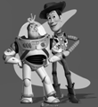
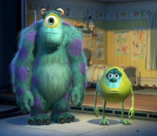
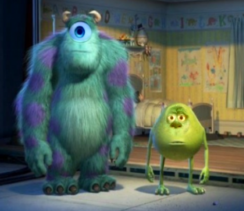
Mike and Sully

I thought it would be fun to swap the eyes of two of my favourite pixar characters Mike and Sully. This is my favourite blending results of the ones I tried. This is because one can clearly see the advantages of using Poisson Blending over just a naive blend. Even with a generous border around the eyes, Poisson Blending is able to make an almost seamless transition. I also find the results quite funny.

Source and Target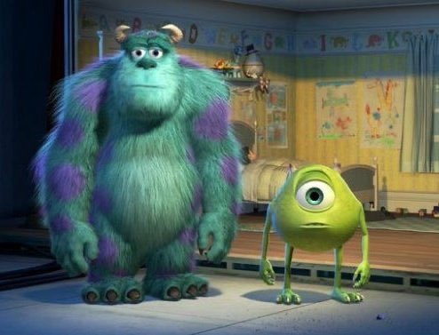

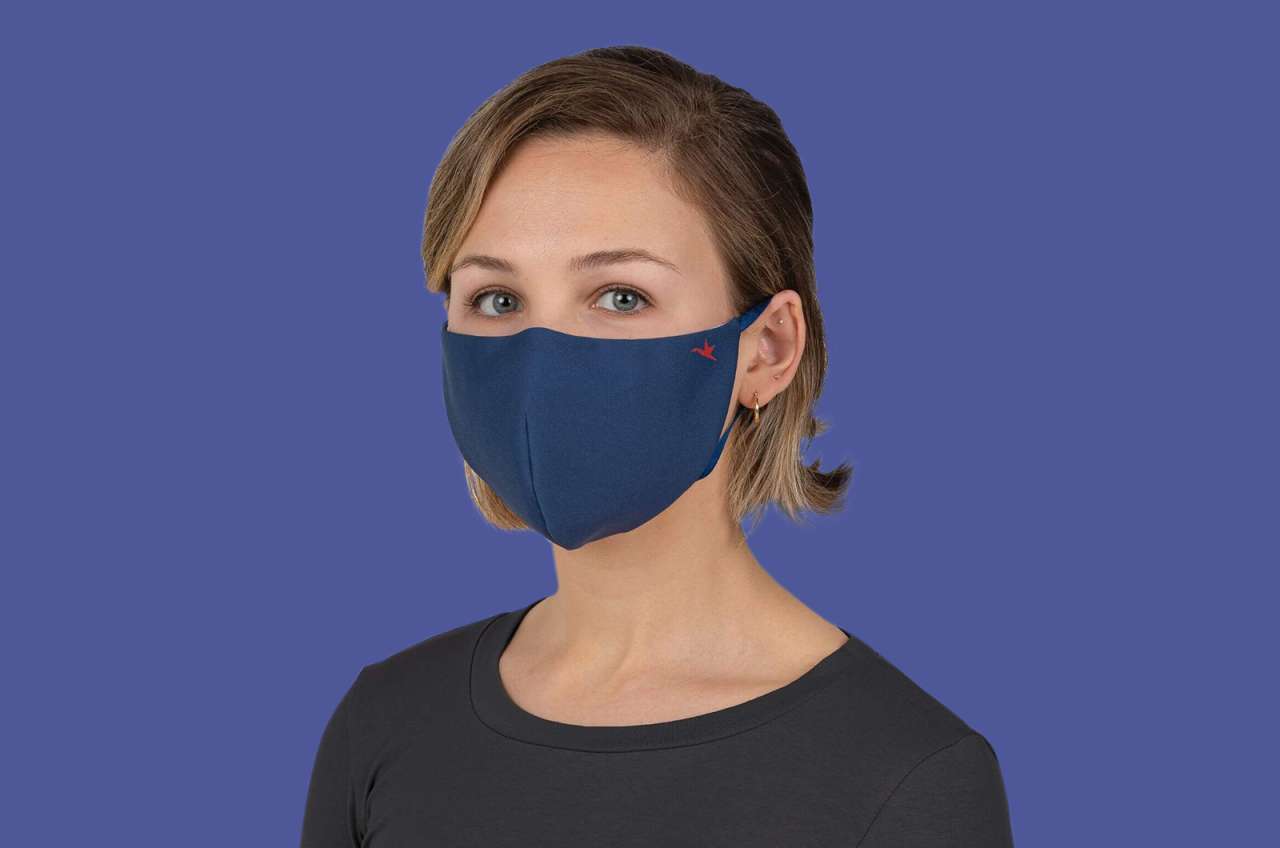
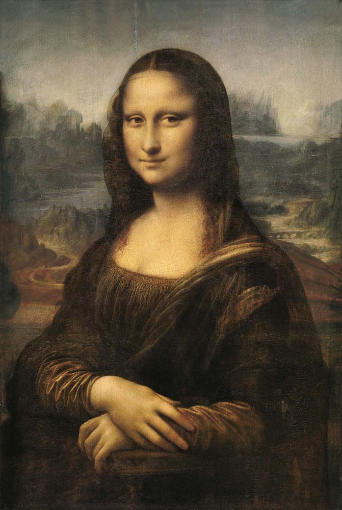
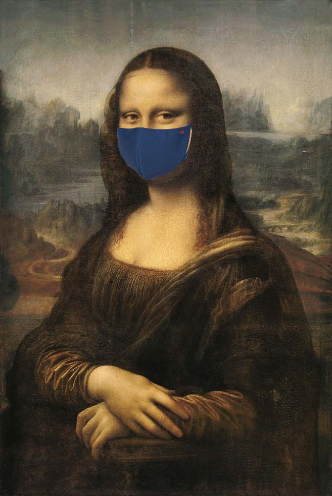
Mona Lisa's Hidden Smile

Everybody love's the Mona Lisa's smile; however, during COVID, it is not really appropriate for her to be out in public not wearing a mask. So I blended a mask onto the famous painting.

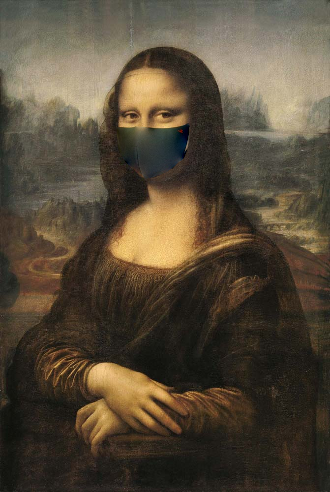
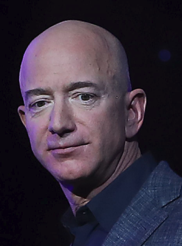
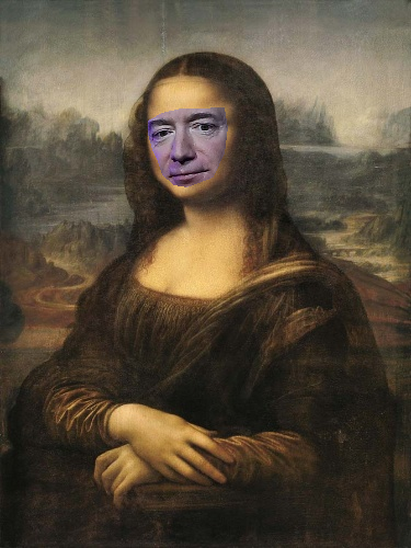
Mona Lisa's New Smile

I came across a photo of Jeff Bezos looking in a similar picture of the Mona Lisa. I wanted to see what would happen if I blended his face onto hers. Turns out it looks like she ages quite a bit.

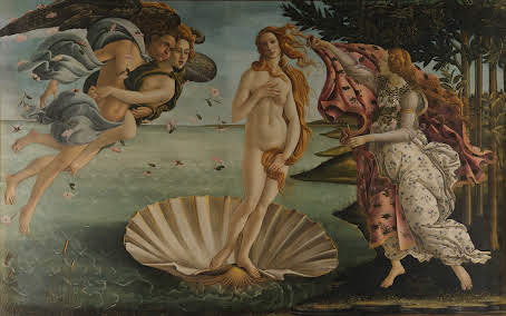
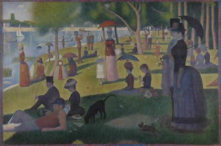
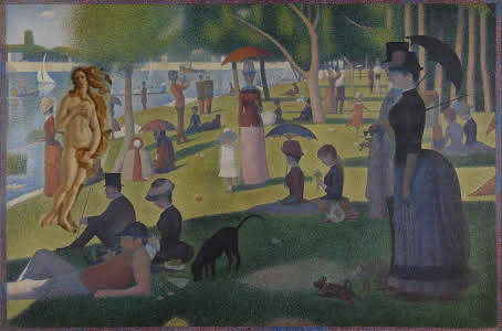
Venus in the Park

I thought it would be interesting to see what would happen if I combined The Birth of Venus with A Sunday Afternoon on the Island of La Grande Jatte.

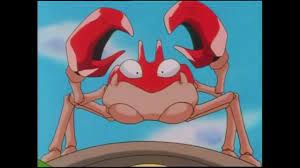
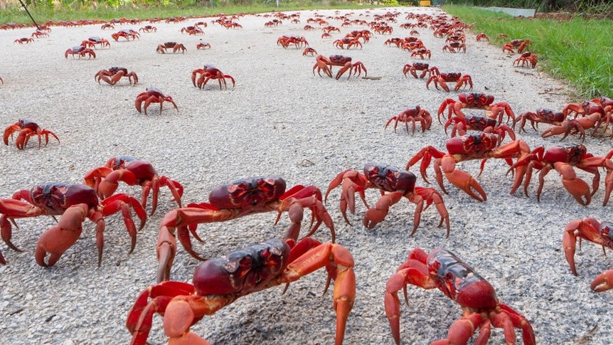
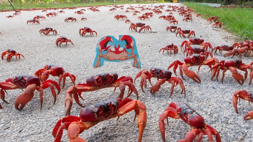
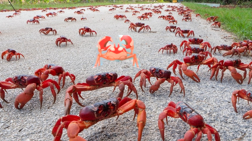
One of these is not like the other (Failure)

I attempted to blend the pokemon Krabby in with a bunch of crabs. However, the results did not look great. The blue in the Krabby background still stands out. This is because the gradient is zero in that area, and that area is in the mask. As a result the Poisson Blending objective tries to keep a consistant colour in the blended image making it look unrealistic.

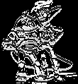
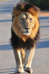
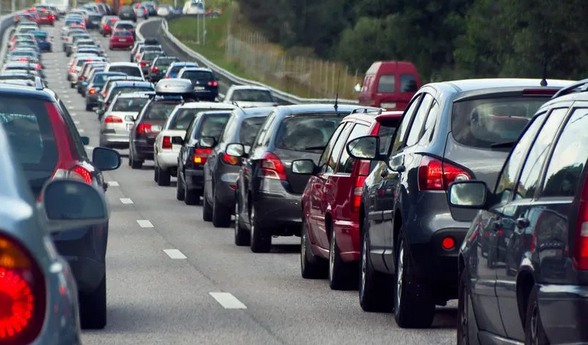
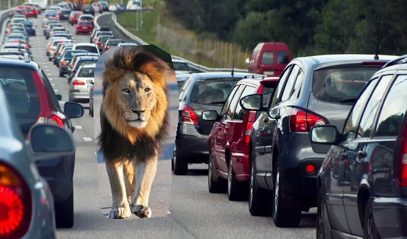
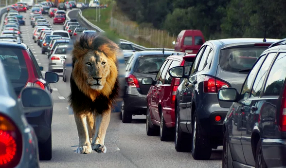
LION!!! (Failure)

I attempted to blend a lion into rush hour traffic. There is a quite distinct blur in the background. This failed because even though the lion is on a road, the texture in the images are too different.

Mixed Gradients

Here, we will slightly modify our least squares objective to instead use the gradient of the source or target with the larger magnitude, represented by "dij" in the equation below.

Below are some examples.

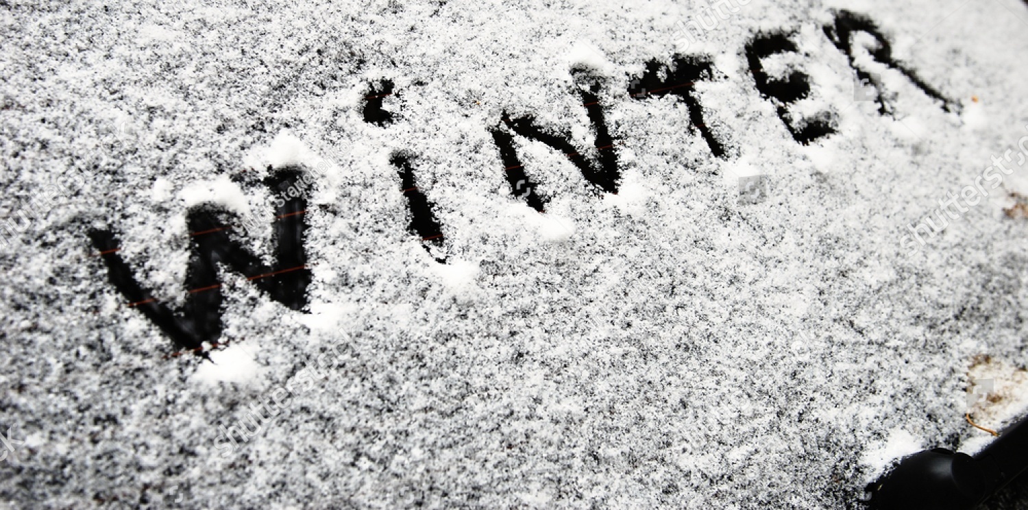
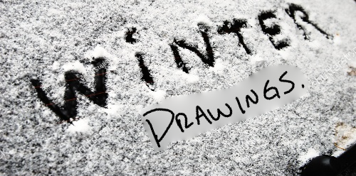
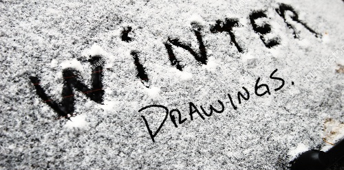
Whiteboard to Snow

Here, we transfer text written on a whiteboard into snow. I only copy the word "drawings".

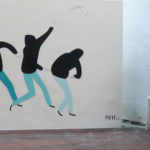
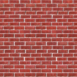
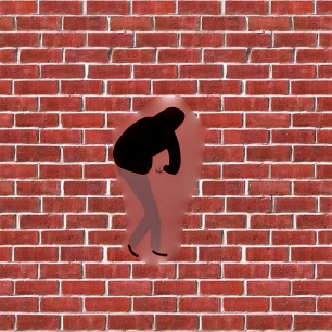
Graffiti Transfer

I tried to transfer graffiti written on a white wall to a brick wall. Mixed performs much better than non-mixed.

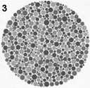
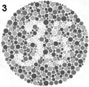
Colour2Gray

Sometimes when converting colour to grayscale, contrast information is lost. This results in the grayscale image being difficult to interpret compared to its original RGB form. To fix this, we can apply gradient domain processing.

Let us look at the example below. The number is not very visible in the grayscale converted image. To fix this, we can first transform the RGB image into the HSV space. This stands for hue, saturation, and value, and is more representative of how human's see images. Hue is the colour of the image, saturation is the strength of the hue, and value is the overall instensity. We have broken up these indivdual channels below.

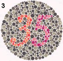
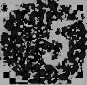
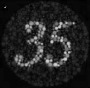
Clearly the v channel resembles similar to what we want. And this makes sense as the v channel represents intensity, which is what we want to capture in a grayscale image. We can therefore us the v channel in our least squares objective. We set the v channel as our target as we want to try to preserve the intensity values, and use the rgb2gray channel as our source because we want to capture those changes across pixels.

There was one more change I had to make to get this to work. As discussed in Poisson Blending, I experimented with adding one objective per direction per pixel vs combining all directions into one objective per pixel. For this task, because I am effectively applying gradient-domain processing on the entire image, I was running out of memory when using one objective per pixel-direction. Therefore, I had to combine the pixel-direction objectives. This turned out to be okay because the processing time was much faster compared to Poisson Blending.

Below are the results of my final implementation run on some images.

Colour Transfer

We implemented colour transfer based on Color Transfer Between Images. How it works is we first convert the source and target images into the LAB space. We use the LAB space because the lowest correlation of channels, allowing for effective colour transfer. We then find the mean and standard deviation of all channels in both images. We do this because we want to change the distribution of each channel in the source to that of the target. This is done by normalizing all the source channels by subtracting the mean and dividing by the standard deviation, and then applying the target's distribtuion by multiplying its standard deviation and adding its mean. The results are some pretty nifty looking photos.

Houses and Hats

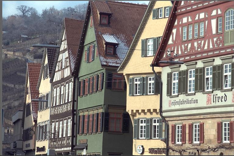
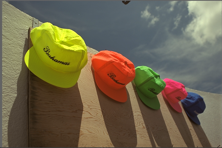
Colour Transfer

Mountains and Space

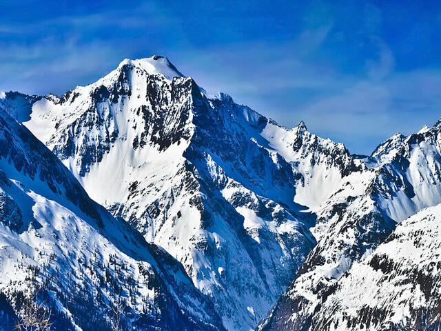
Colour Transfer

Islands

Colour Transfer

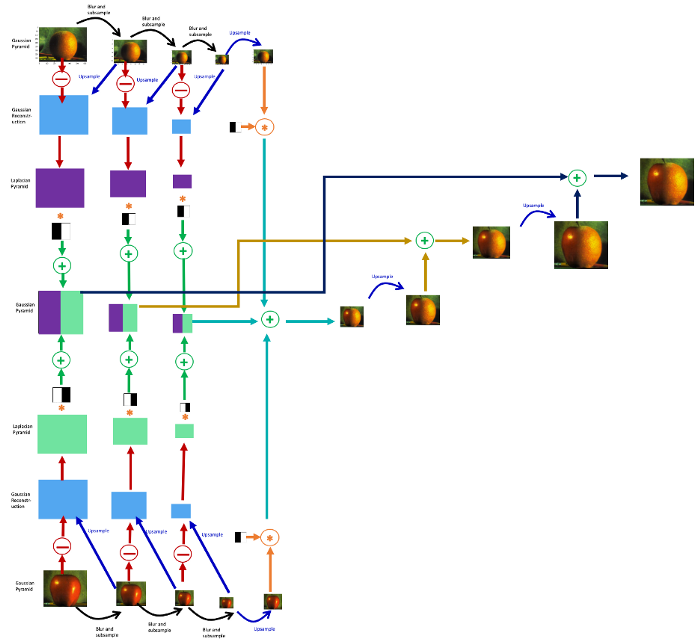
Laplacian Pyramid Blending

Laplacian Pyramid Blending is another tool that can be used to blend objects in images. It can blend the boundary of the objects while keeping the surrounding area intact.

Laplacian Pyramid Blending builds off the image pyramid we learned in our last assignment. We build the Laplacian Pyramid by first constructing a Gaussian Pyramid. For each pyramid level, the image gaussian smoothed and then downsampled by a factor of 2. Then, to construct the Laplacian, each level in the Gaussian Pyramid level is upsampled and subtracted from the Gaussian Pyramid level above it. The Gaussian filters captures the low frequency content at each level of the pyramid, and the subtaction captures the difference, making it theoretically possible to restore the original image.

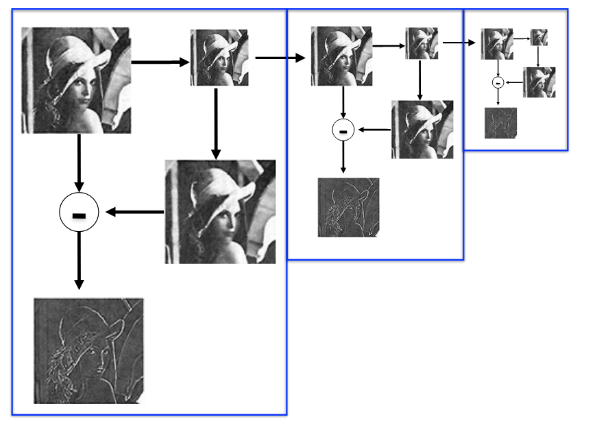source: http://16720.courses.cs.cmu.edu/lec/filters_lec2.pdf>

For Laplacian Pyramid Blending, we build the Gaussian and Laplacian filters for both images. Then, at each pyramid level, the laplacians of the two images are combined, upsampled, and added to the previous level, repeating up the pyramid.

source: https://becominghuman.ai/image-blending-using-laplacian-pyramids-2f8e9982077f

Instead of just blending half of one image with the other, I specify a mask so that we can use the same blending infastrucutre for Poisson Blending. The result is a blended image with a smooth transition in the middle.

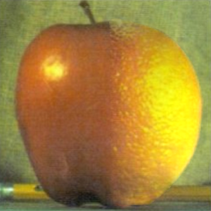
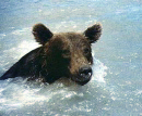
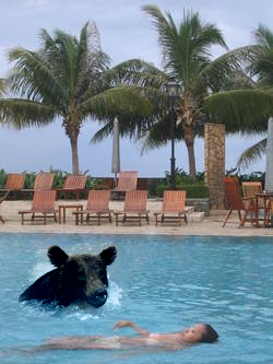
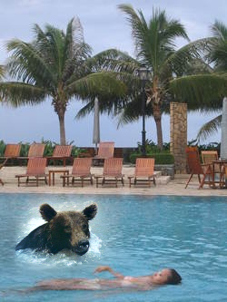
As we can see in the below examples, Laplacian Pyramid Blending provides a smoother transition than Poisson Blending. As well, it does not really affect the colour of the source image, which is quite noticeable in the bear in the water. However, Poisson Blending does a better job at matching the colours along the boundary of the mask.

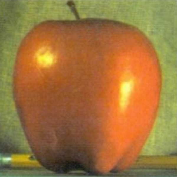
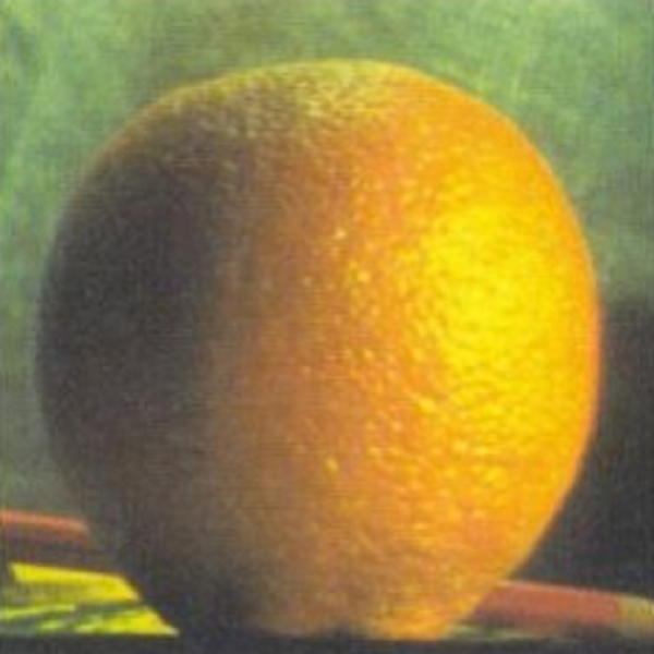
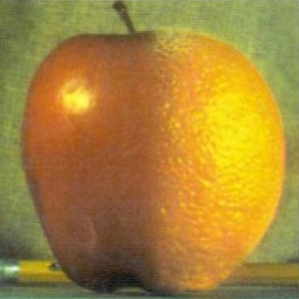
Apple and Orange

Bear in Water

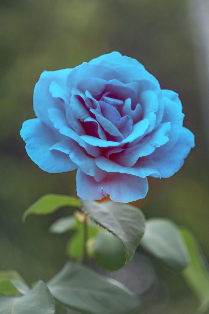
Laplacian Colour Chnages

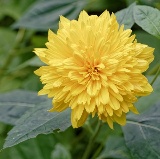
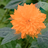
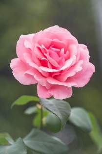
As described in Poisson Image Editing, Poisson Editing can be used to manipulate colours in images. One example is local colour changes. This is very similar to Poisson Blending. The boundary is defined in the image, and the least squares objectives are to keep the colour the same at the edges of the boundary, while keeping the gradients within the same with an adjusted colour value. Below are a couple results on flowers.

Yellow to Orange

Pink to Blue

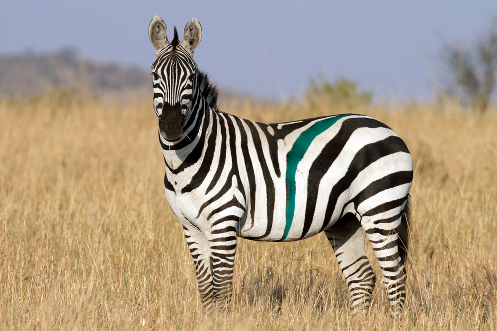
As well, here is a Zebra with a single stripe changed to green.

Conclusion

Gradient domain processing is a powerful tool when it comes to image manipulation. Combined with colour space transformations, many creative ideas are now easily manageable. Further ideas I would have liked to explore are non-photorealistic rendering, poisson flattening, and poisson sharpening.