Single Scale NCC

The first step was to be able to reproduce small-scale, low resolution images. To do this, we make the assumption that the three images to be aligned all represent a specific RRB channel (this may not be true for all images). We also assume that the offsets in the channels are a pure translation, with no rotations ( again, this may not be true across all images).

We set the objective to be to align both the red and green channels with the blue. The easiest way to allign the channels is to perform an exhaustive search over a specified window. For each combination of horizontal and vertical displacements in the window, an image similarity metric is measured. The horizontal and vertical shift combination with the best image similarity metric is used as the final translation for that channel.

Three image similarity metrics were evaluated. Sum-of-squared differences (SSD), Normalized Cross Correlation (NCC), and my own gradient implementation discussed in BW Grad. While all three performed almost equivalently for the low resolution images, I ended up selecting NCC because it scaled better when implementing Image Pyramid NCC. As well, the window size I used was [-15, 15] for both horizontal and vertical displacements, resulting in a total of 961 combinations to evaluate (2*15+1)^2.

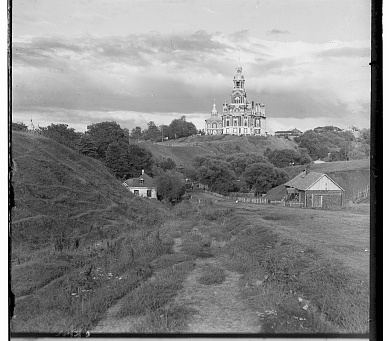
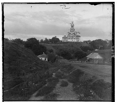
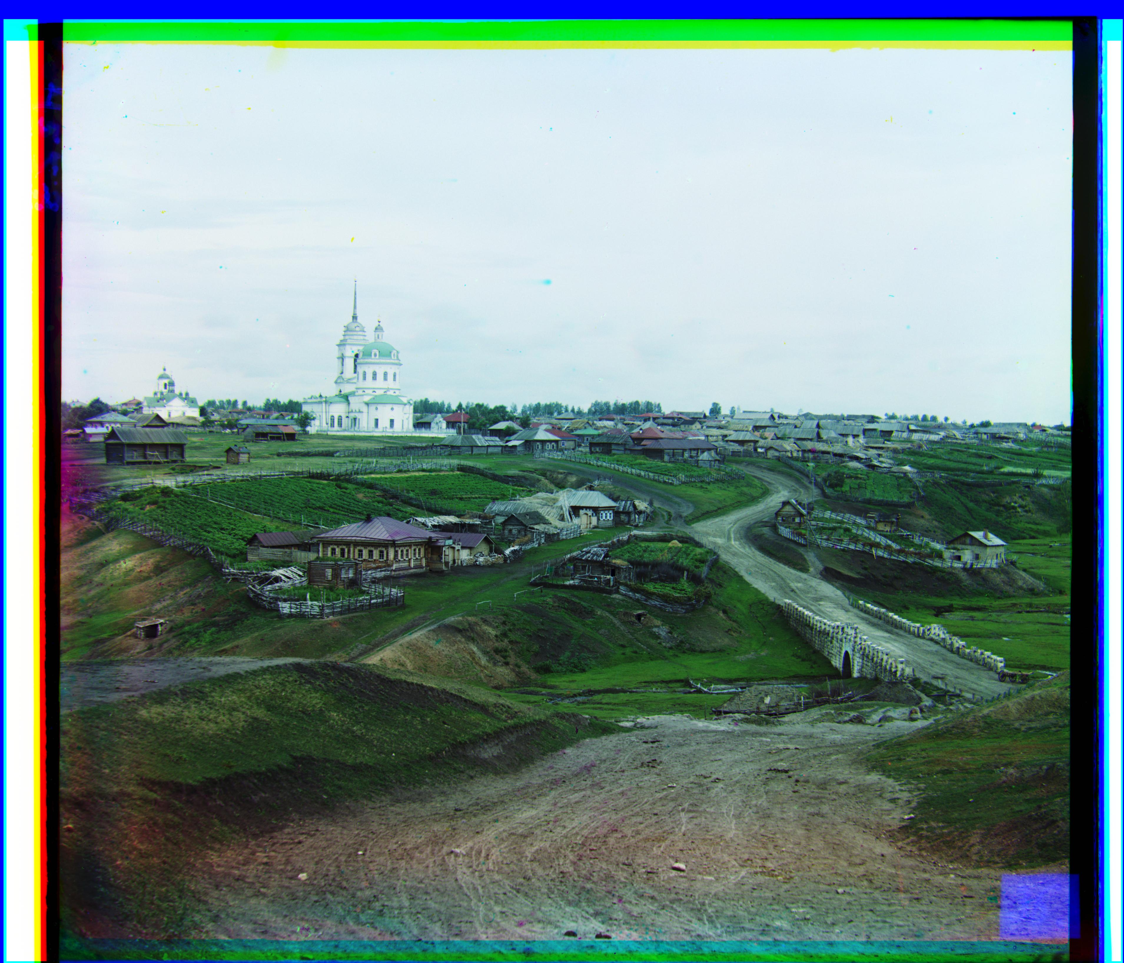
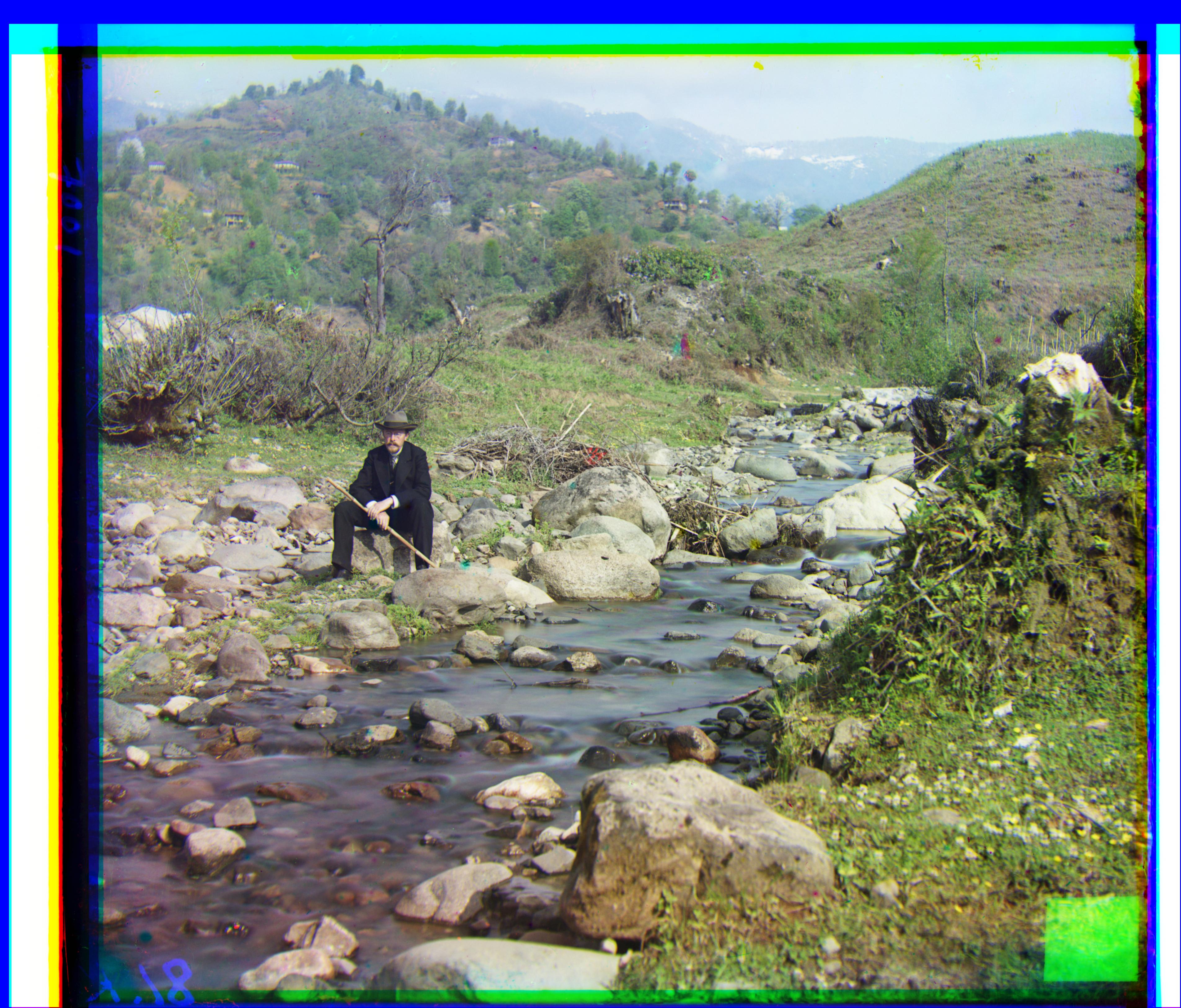
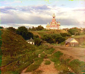
Below is the result after finding the best translation for the red and green channels.

Restored Image - r_shift: (3, 12), g_shift: (2, 5)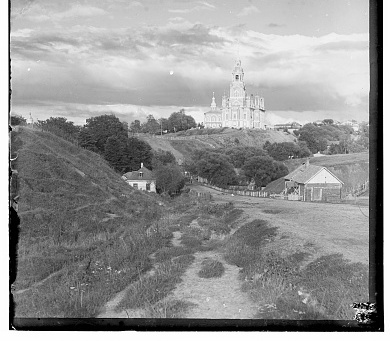

While this method is promising on low resolution images, it impratical for higher resolution ones. This is because the search across all displacements will become more and more expensive as the image size increases. If we decrease the window size, then the best shift may fall outside the window. Therefore, another solution is needed. We address this issue in the next section Image Pyramid NCC.

Image Pyramid NCC

Next, we will implement an image pyramid as a faster search procedure to align the images. An image pyramid represents the image at multiple scales. Each level of the pyramid is the image scaled down to a lower resolution. We then process the small pyramid level first and work our way up to the largest image, updating our shift estimate at each level. The advantage of this is that we do not need to have a large search window for large scale images. Smaller image levels can have larger search windows where it is computationally less expensive to get an initial translation approximation, and larger image levels will have smaller search windows where the approximation is refined.

Image pyramid example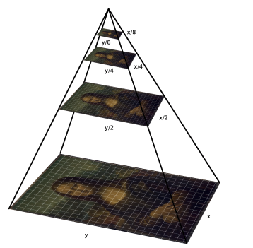source: https://iipimage.sourceforge.io/documentation/images/

In my impelementation, each pyramid level is scaled by a factor of two. To get the number of pyramid levels, we take the log2 of both smallest image dimension and user defined input specifying the smallest size of the smallest pyramid level (I used 128). The number of pyramids is determined to be the number of levels it takes to reach that size. Lastly, at the smaller sized pyramid levels, the window size is again [-15, 15]. Howewer, at the larger levels, the size decreases to [-5, 5] to improve speed.

As in Single Scale NCC, the same three image similarity metrics were evaluated. However, this time there was a noticeable difference between the three. SSD performed the least well upon visual inspection. Our gradient based implementation in BW Grad, while performing the best, was a little slower (3-5 minutes compared to under 1 minute for NCC). Therefore, NCC was selected.

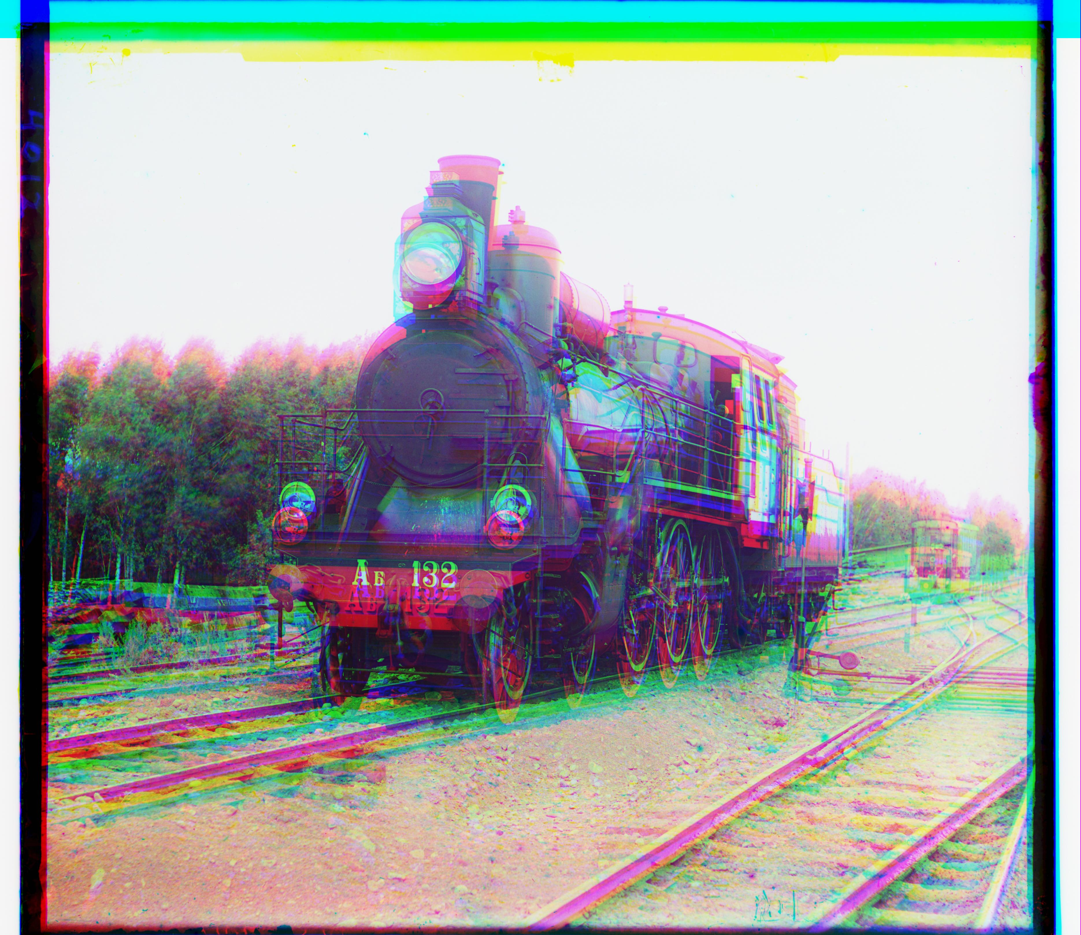
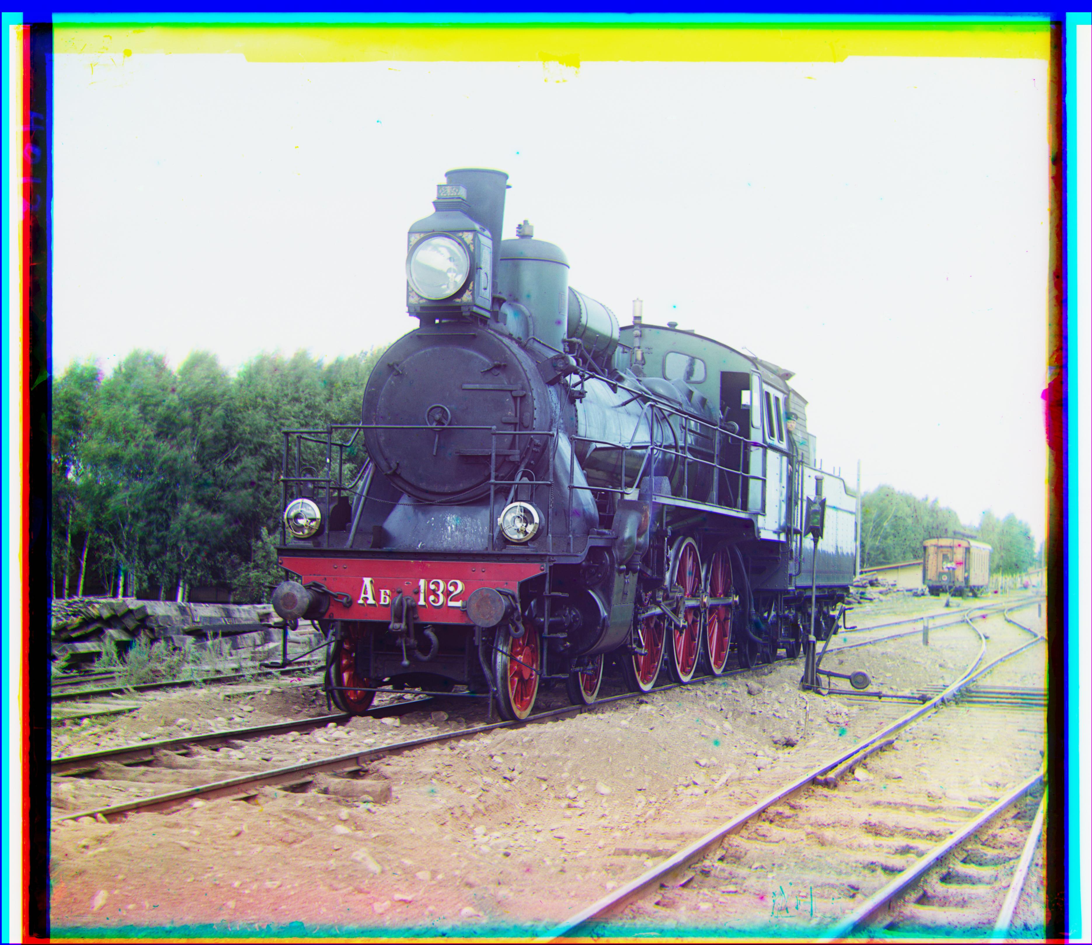
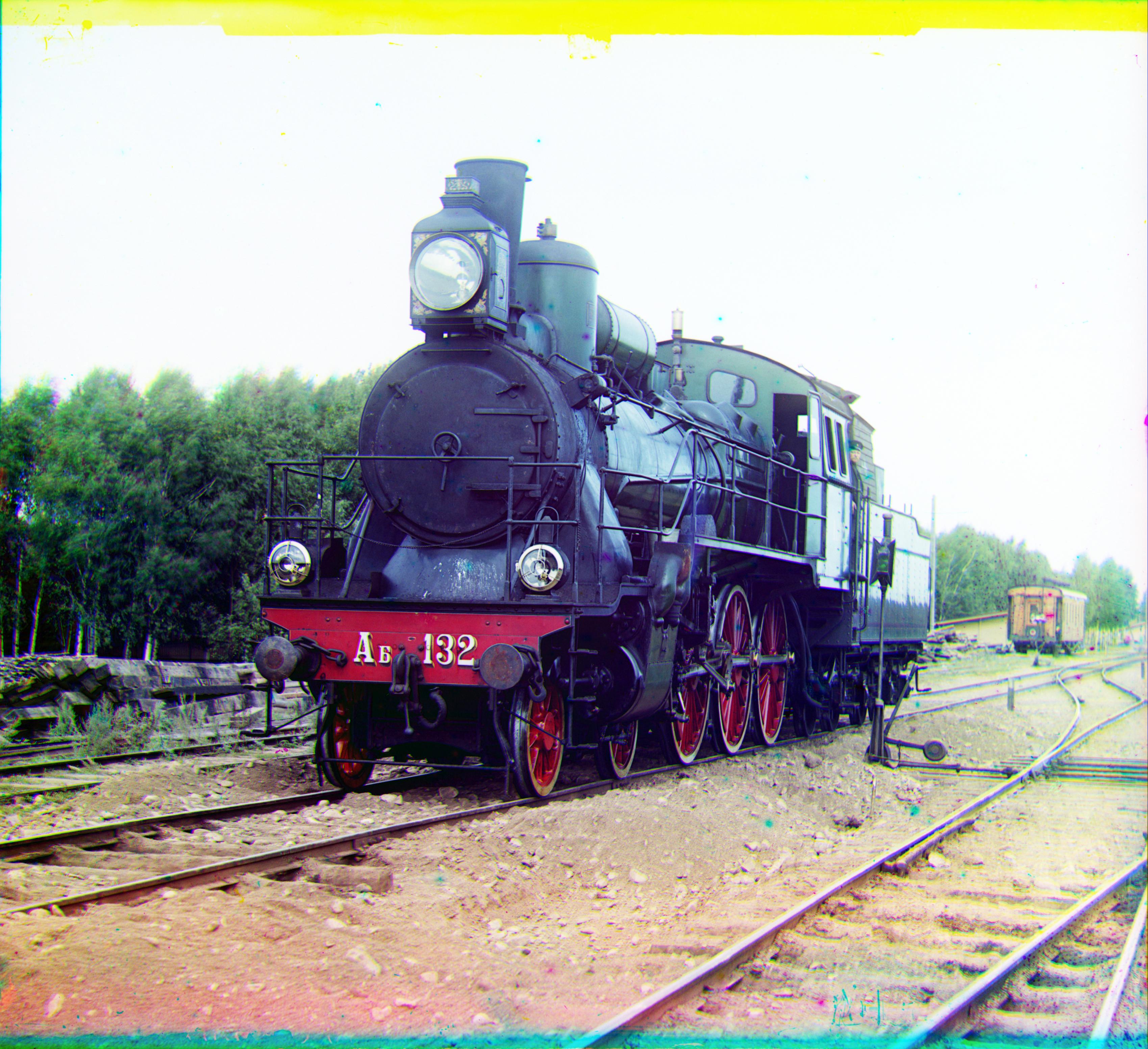
There was one more issue I had to address. For some of the images, such as train.tif, the alignment was performing very poorly. This turned out to be because of the borders and missing colours that would appear in some channels. To remedy this, I only used NCC on the pixels that fell within 10% of the smallest dimension from the sides of the image. The results looked a lot better. This was also one of the reasons I later ended up implemented automatic border cropping in BW Cropping.

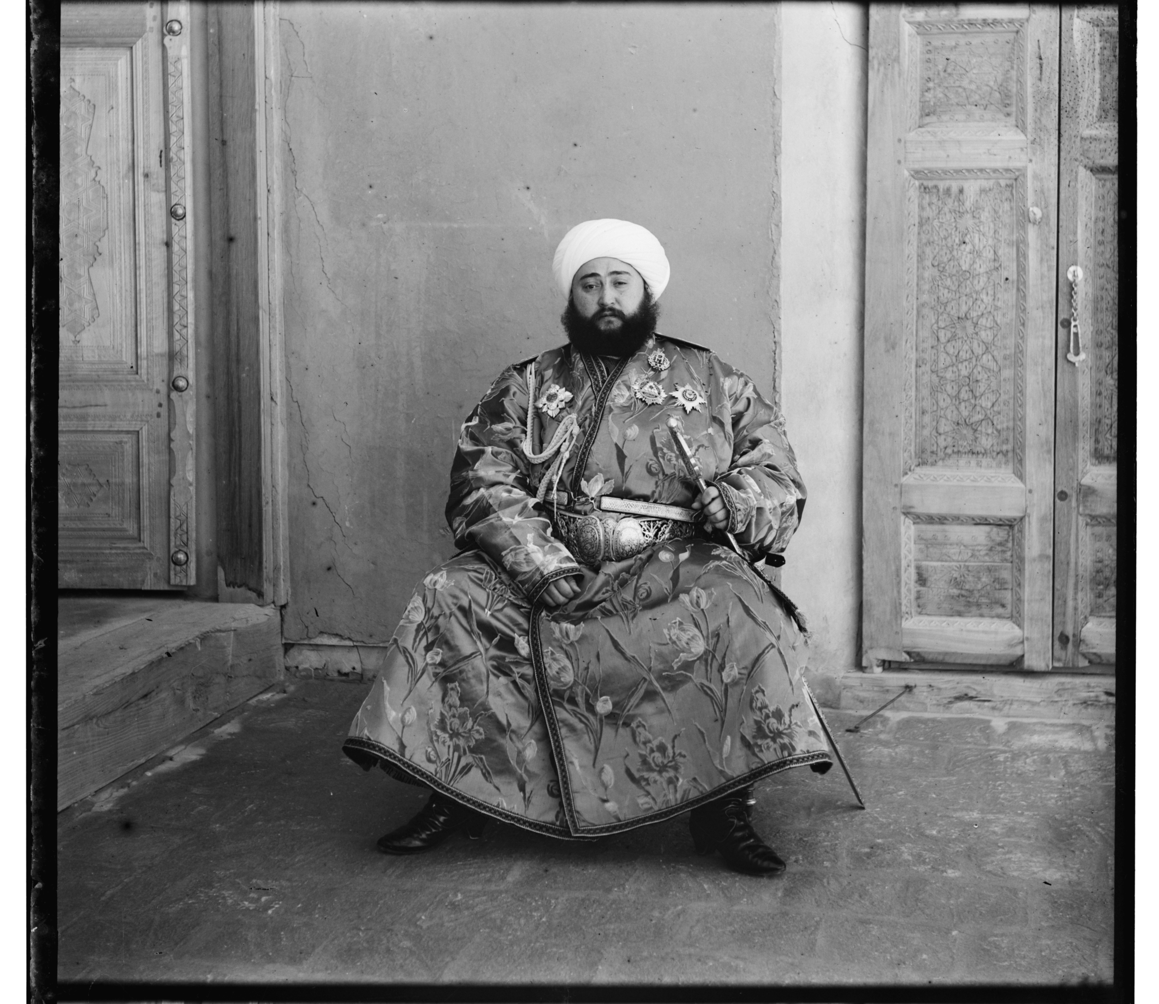
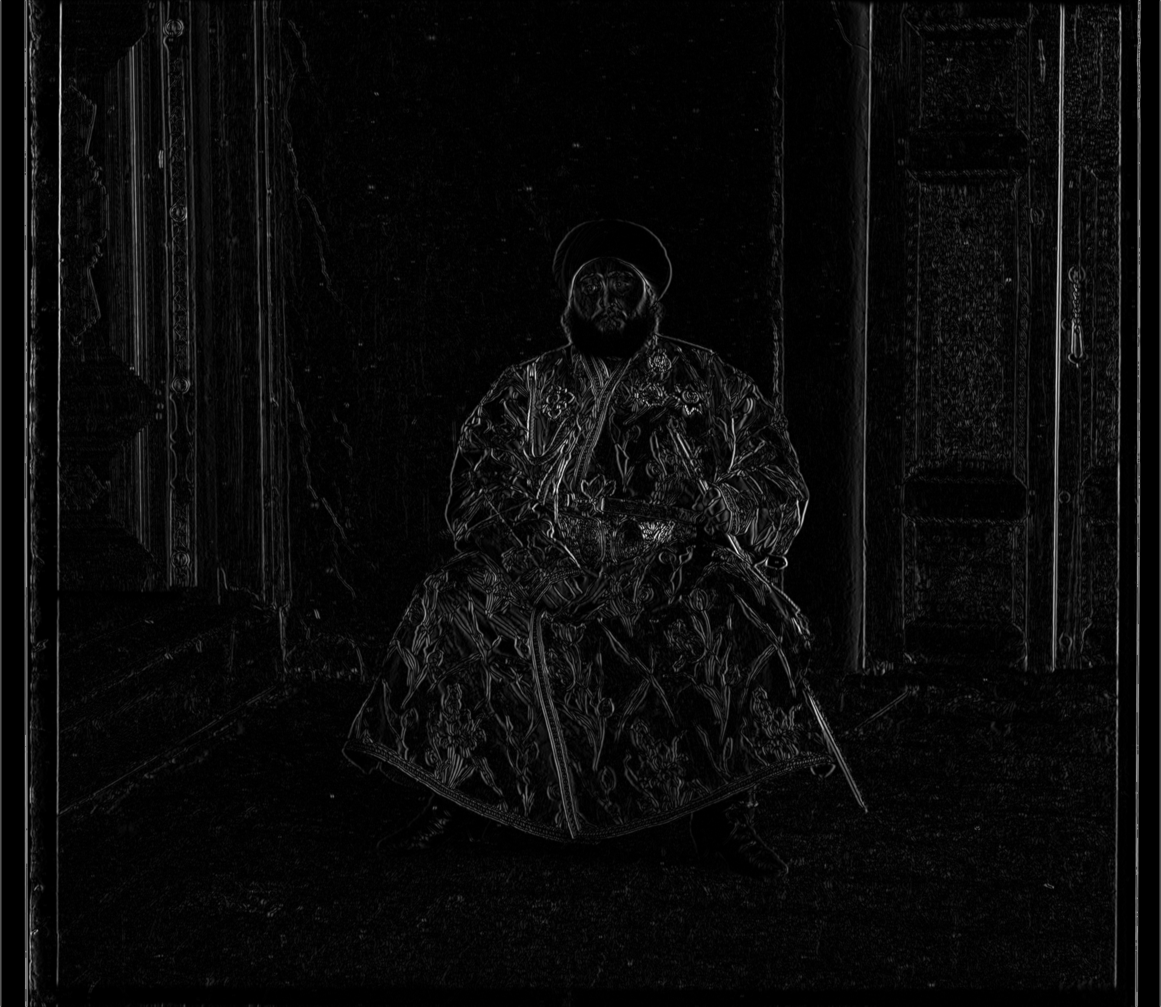
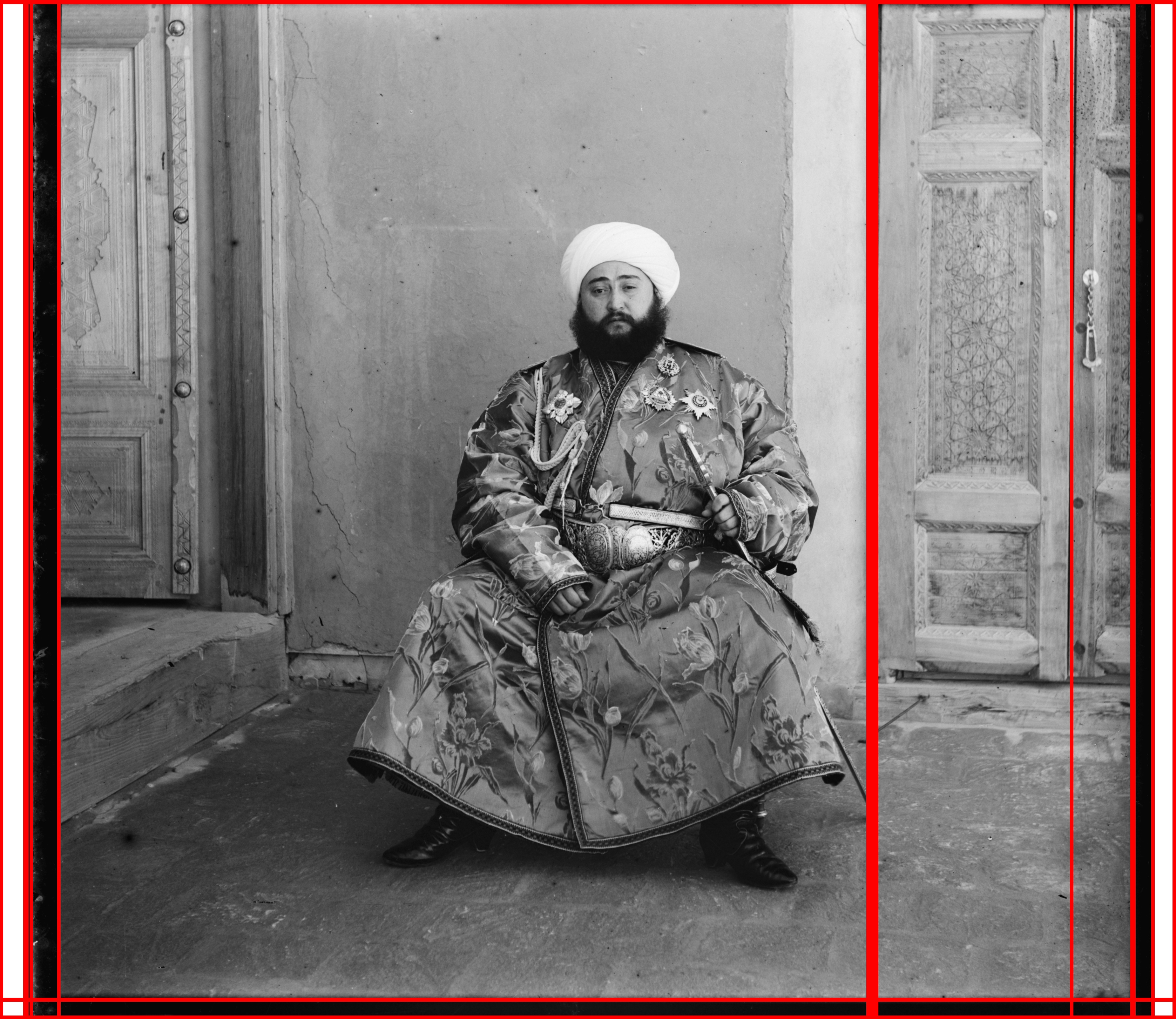
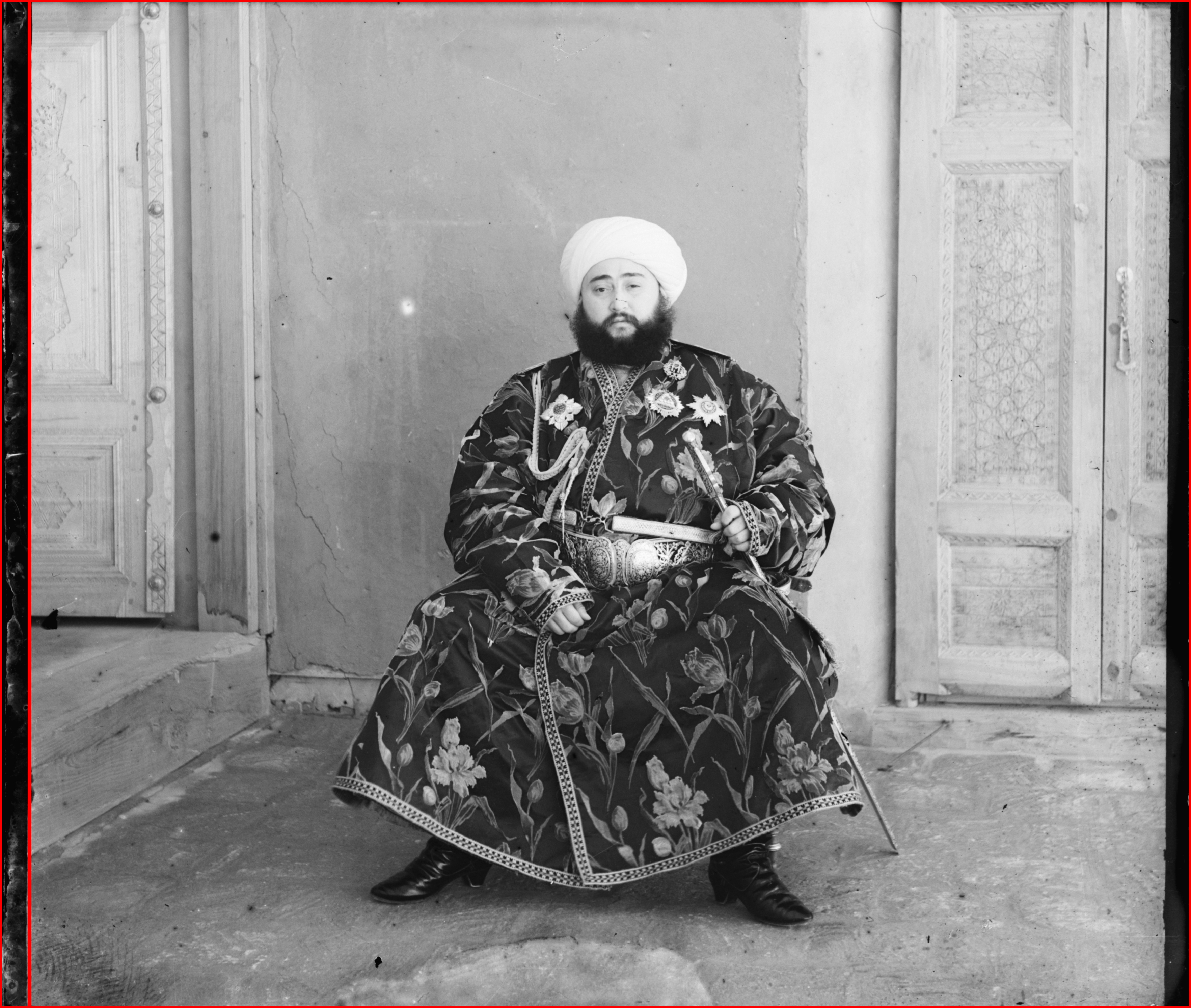
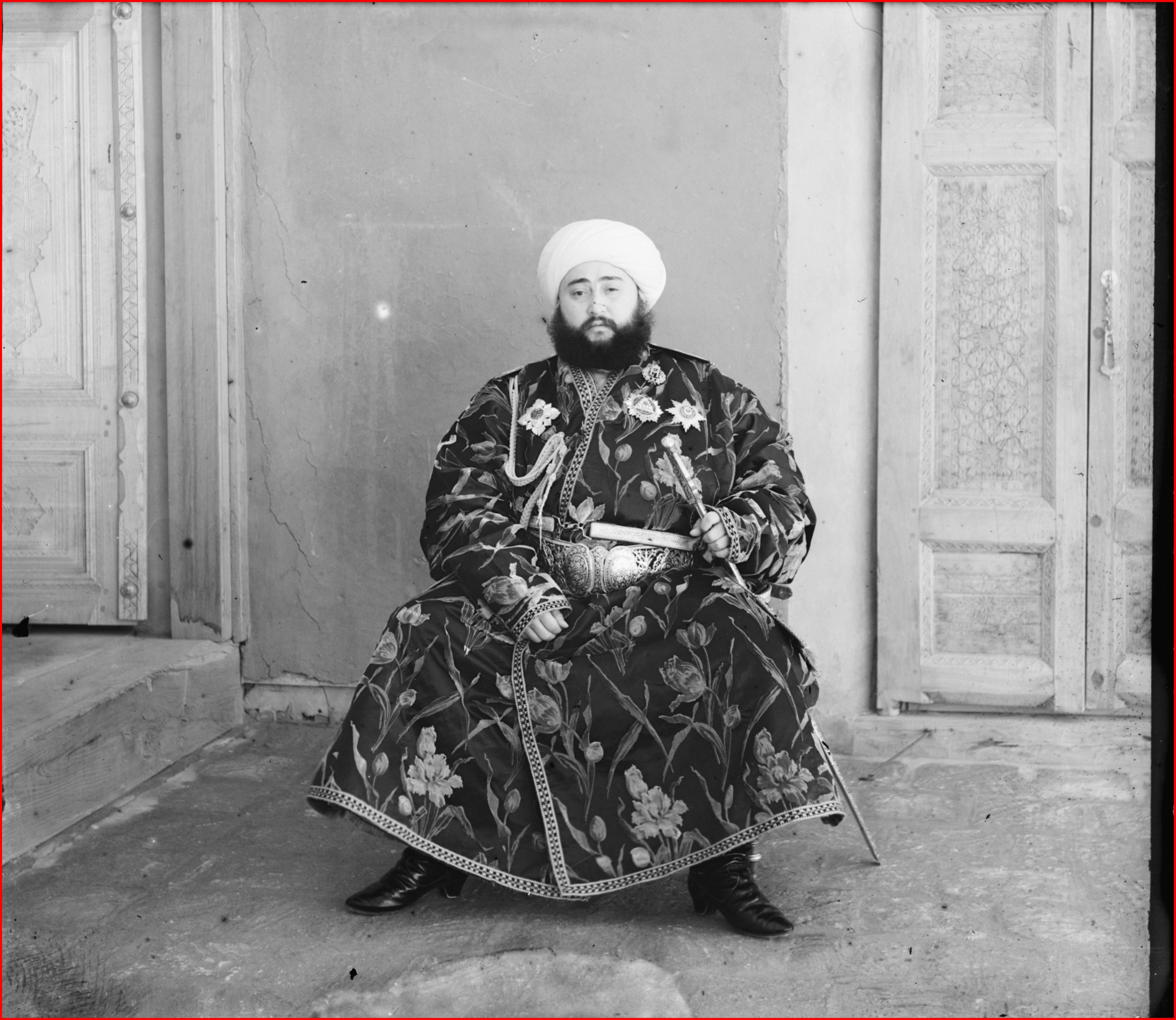
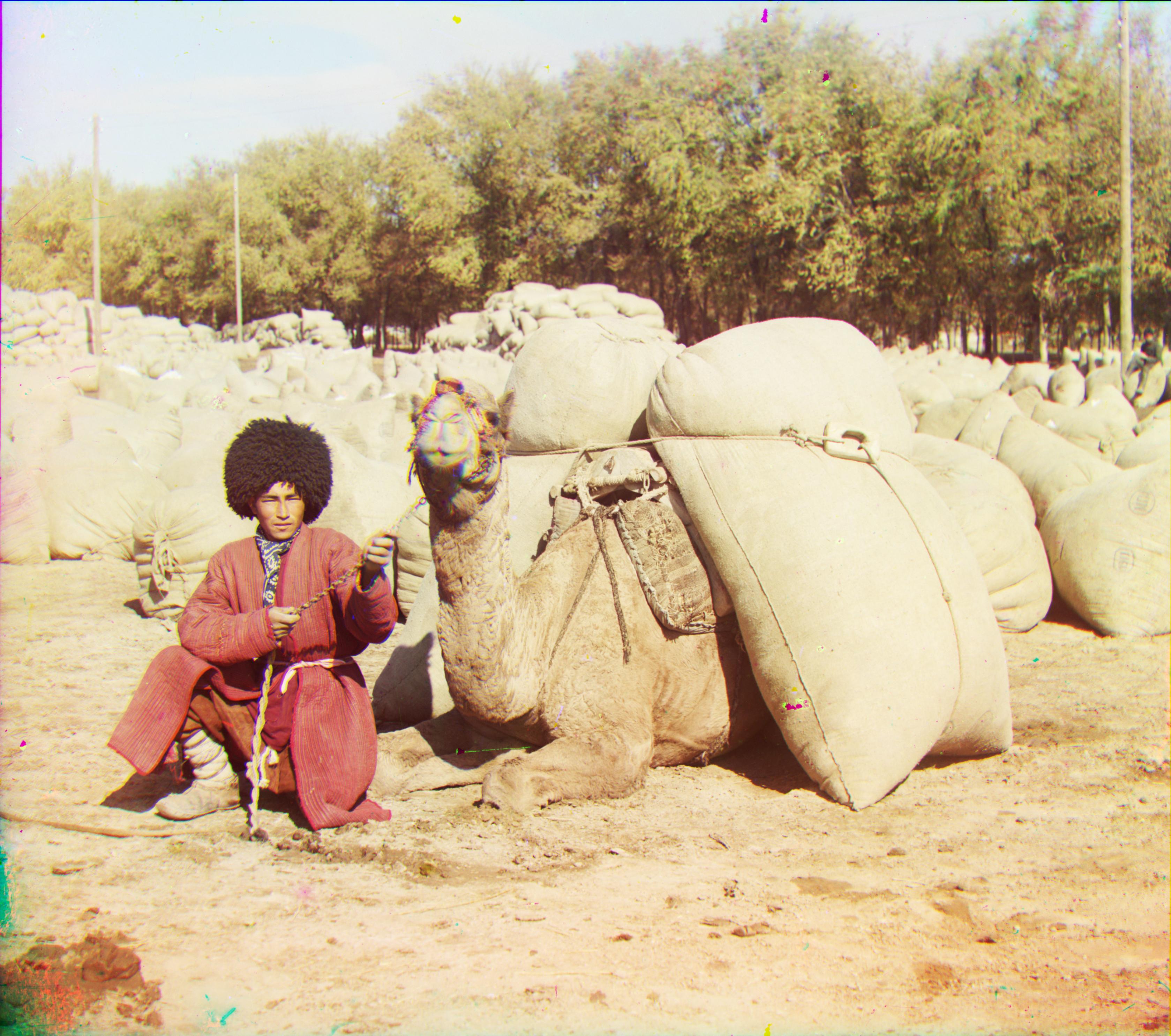
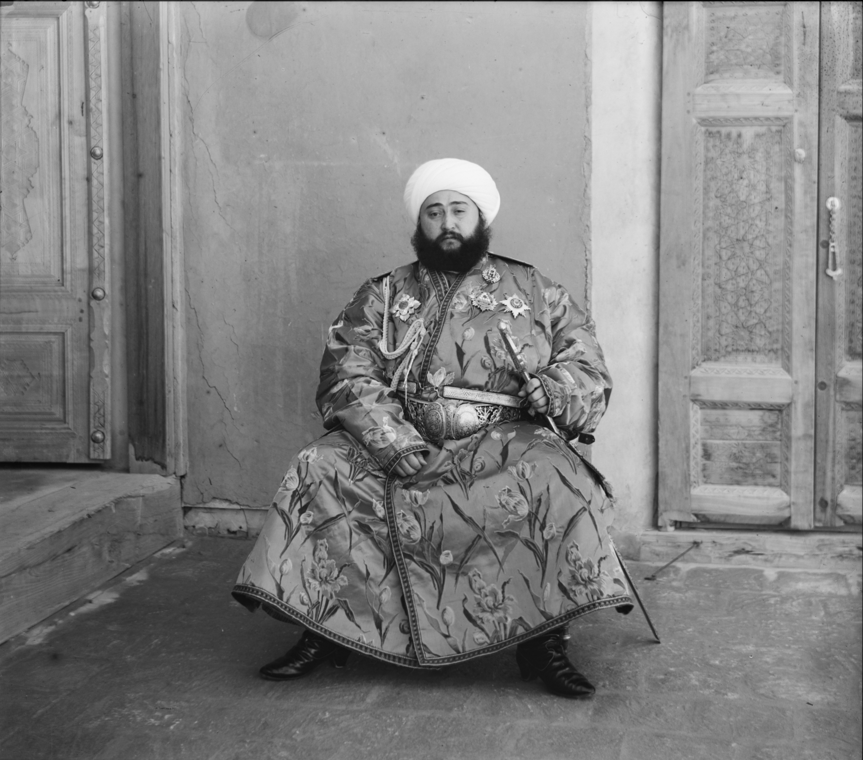
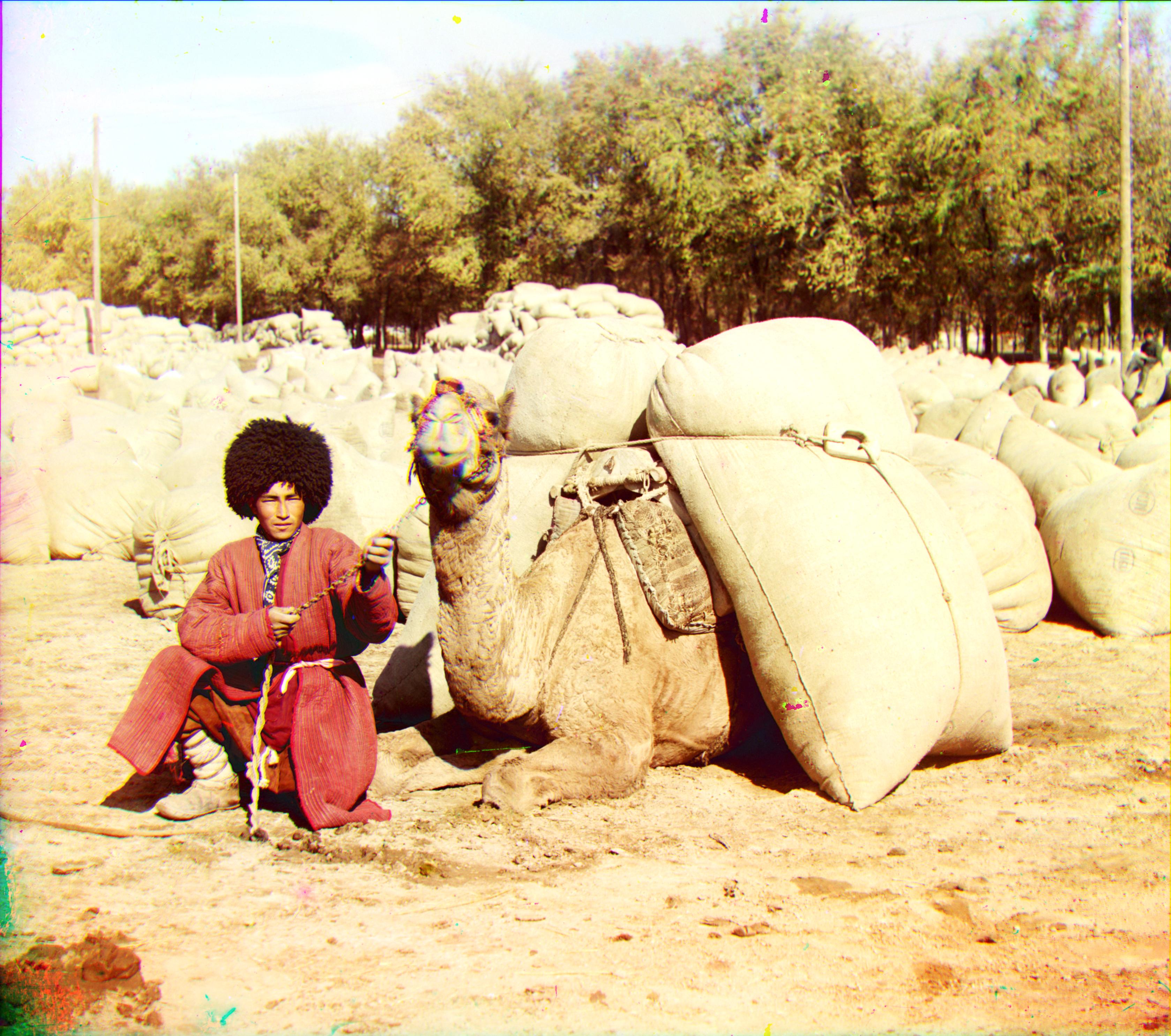
Below is the result after finding the best translation for the red and green channels. The method performs well for all images except for emir.tif. If you look closely, there is some bluriness, particularly around the hand area. This is because the three channels do not have the same brightness levels. As a result, NCC will not perform as well due the brightness level variation. I address this issue in BW Grad.

Bells & Whistles: Pytorch Implementation

For my first Bells and Whistles task, I implemented everything I described above in Pytorch. Not a single numpy or open-cv call is used. The only non-Pytorch libraries used are libraries used for file io. The resulting channels have the same shifts and as a result the output images are exactly the same.

Single Scale NCC

r_shift: (3, 12), g_shift: (2, 5)

Image Pyramid NCC

Custom Gradient Metric

Now comes the fun part. As descbribed above in section Image Pyramid NCC, NCC does not perform well for emir.tif because of the varying brightness across channels. Therefore, we need to modify our image matching metric such that it is brightness invariant.

To do this, I am going to do something similar to what they did in Histogram for Oriented Gradients https://lear.inrialpes.fr/people/triggs/pubs/Dalal-cvpr05.pdf. Specifically, I am going to use the gradients and and calculate a normalized feature vector. However, I am not going to do any of the orientation binning as it is not needed and only slows things down (but I did try it). Also, I am not going to worry about dividing the image into cells and blocks as recalculating those for each pixel shift would be add too much to the runtime. Instead, each pixel will have its own nine sized normalized feature vector which is composed of the magnitudes of the gradients of its nine surrounding pixels.

The first step is computing the gradients of the image. I compute the gradients in both the x and y direction and take the magnitude for each pixel. As they did in HOG, I use a 1D gradient filter. The feature vector for each pixel is then calculated by just concatenating the magnitudes of the gradient of the nine pixels surrounding it. For the pixels on the border, the sides with no surrounding pixels are assigned a magnitude of zero. Lastly, the feature vector for each pixel is normalized.

There are two main reasons why I did this. First, taking the gradient removes average brightness levels across each channel, as we are now only looking at how pixels change. Second, normalizing the feature vectors make the system more robust to variances in illumination and shadowing. If one channel's pixels scale by twice those of another channel's, normalizing the feature vectors will remove this scaling. I felt that these two improvements would be enough to fix the emir.tif issue.

To compare images, I again use the same window displacement values as in Image Pyramid NCC. However, the image metric I use now is the Sum of Squared Differences of each feature in the feature vector for each pixel.

Yet, there was one more optimization I had to do. Because each image comparison now used nine values for each pixel, this implementation was very slow on the larger image pyramid levels. To improve this, I sampled the pixels I would use. At first I tried random sampling, but ran into similar border issues as in Image Pyramid NCC. Instead, I sampled a square area of side length 451 from the centre of the image. This correspondeds to sampling 451*451 = 203,401 pixels. Before iterating over all the possible window displacements, I would sample these pixels to perform the Sum of Squared Differences. If the image was smaller than this size, I would use the entire image.

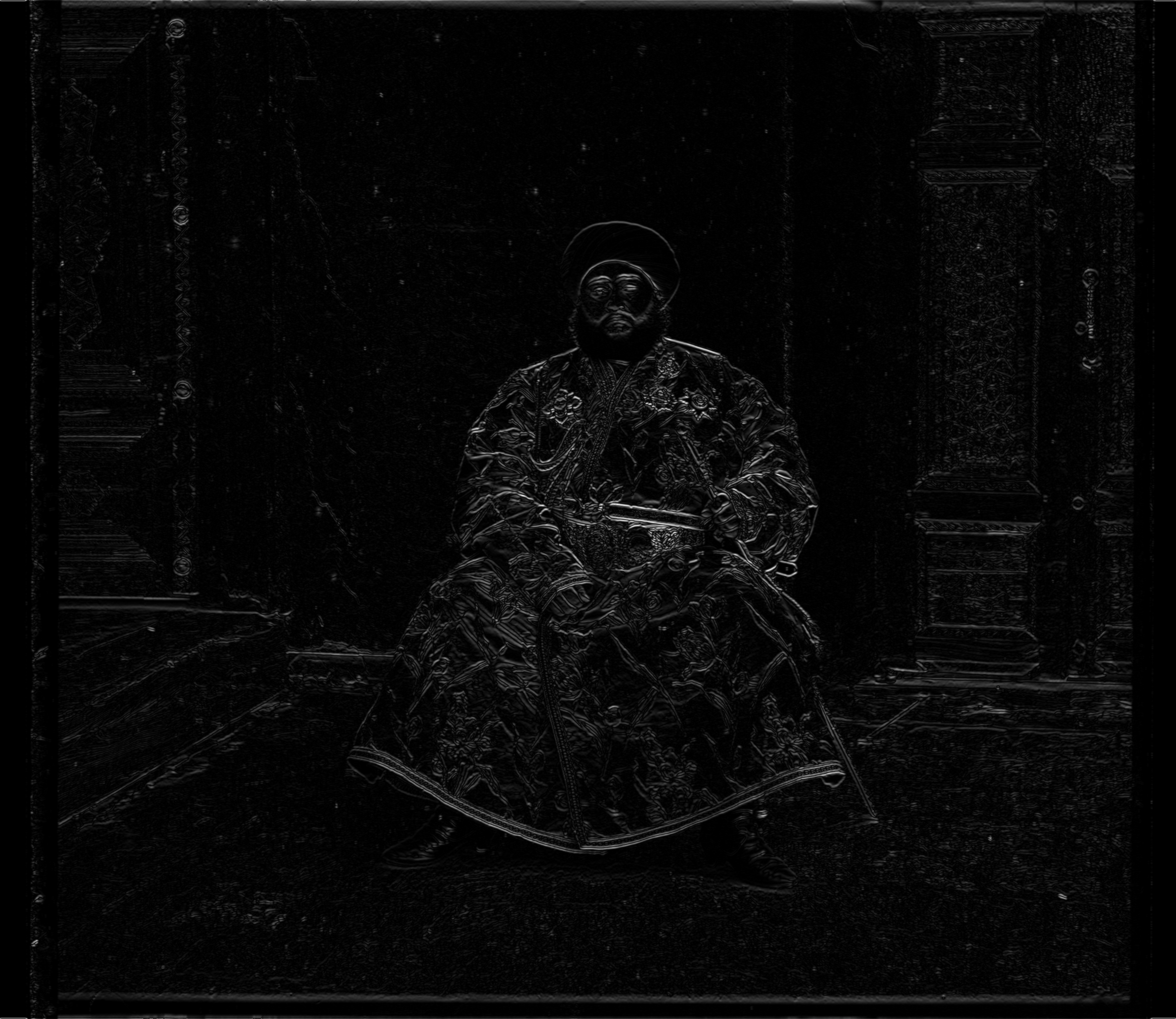
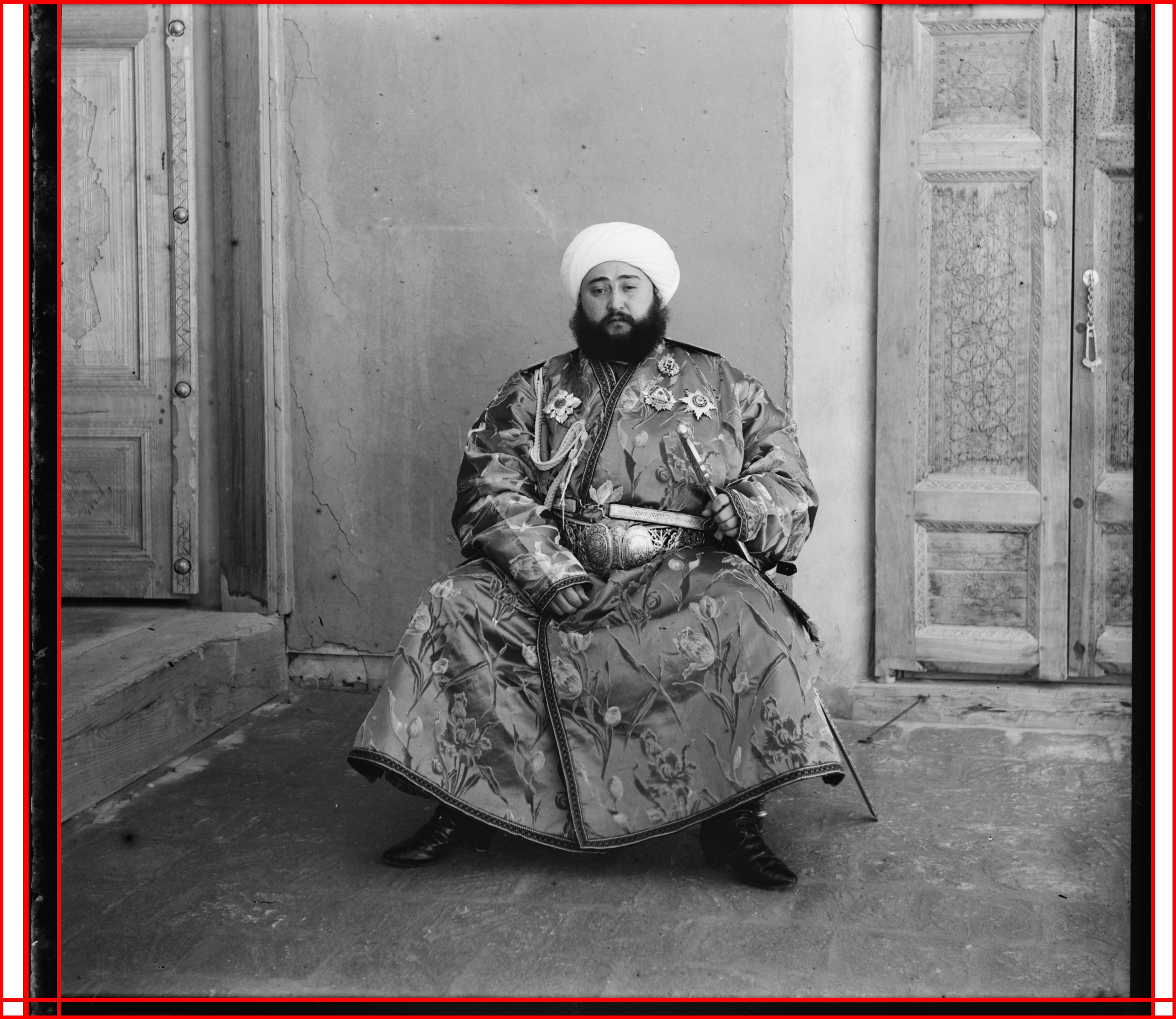
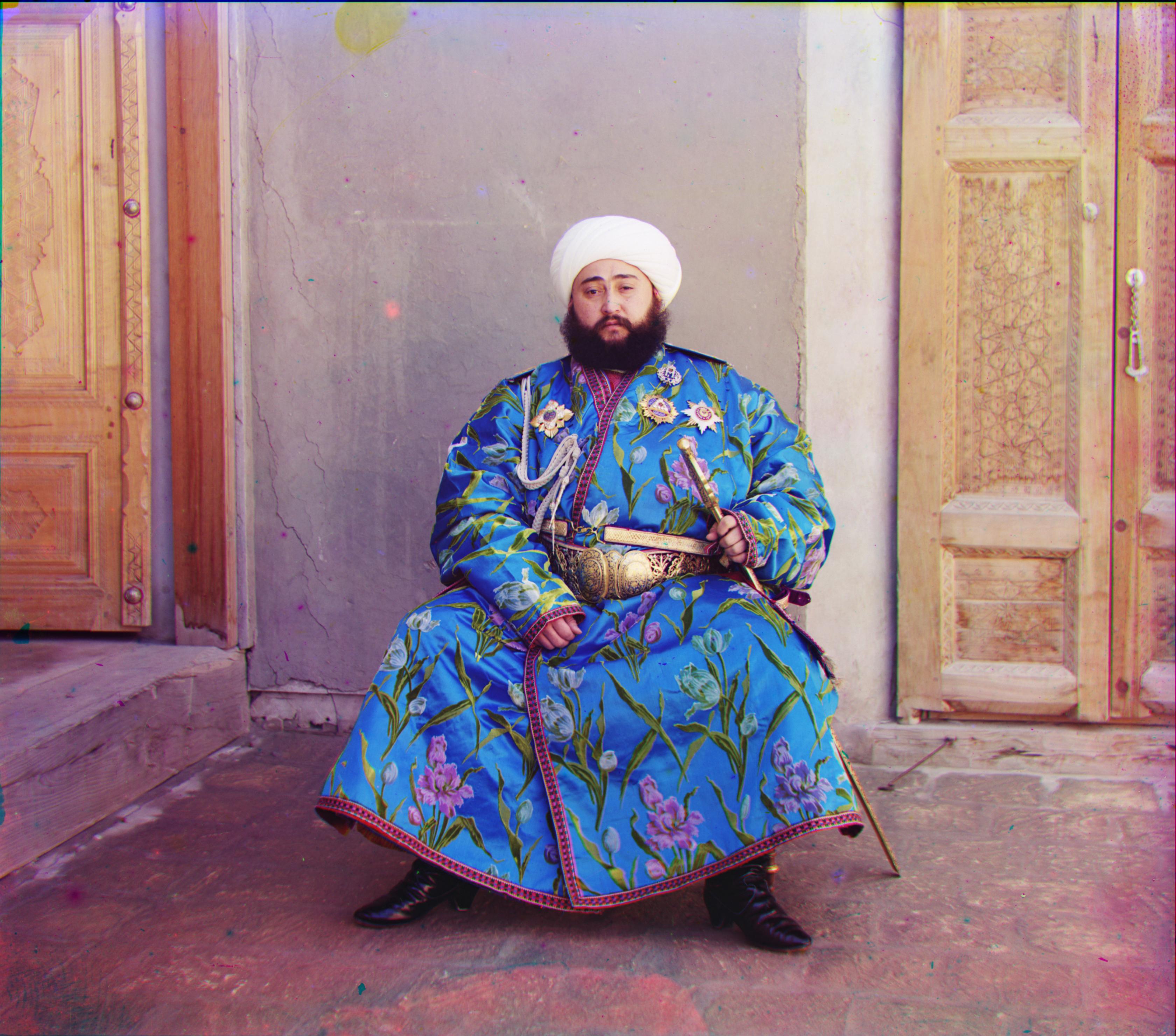
This ended up working very well. There was a significant improvement in the runtime, and at no noticeable cost to performance. Notice the significant improvement for emir.tif. You can no longer notice any major blurs (look at the hand).

NCC Pyramid Alignment - r_shift: (56, 104), g_shift: (24, 49) New Pyramid Alignment - r_shift: (41, 106), g_shift: (23, 48)

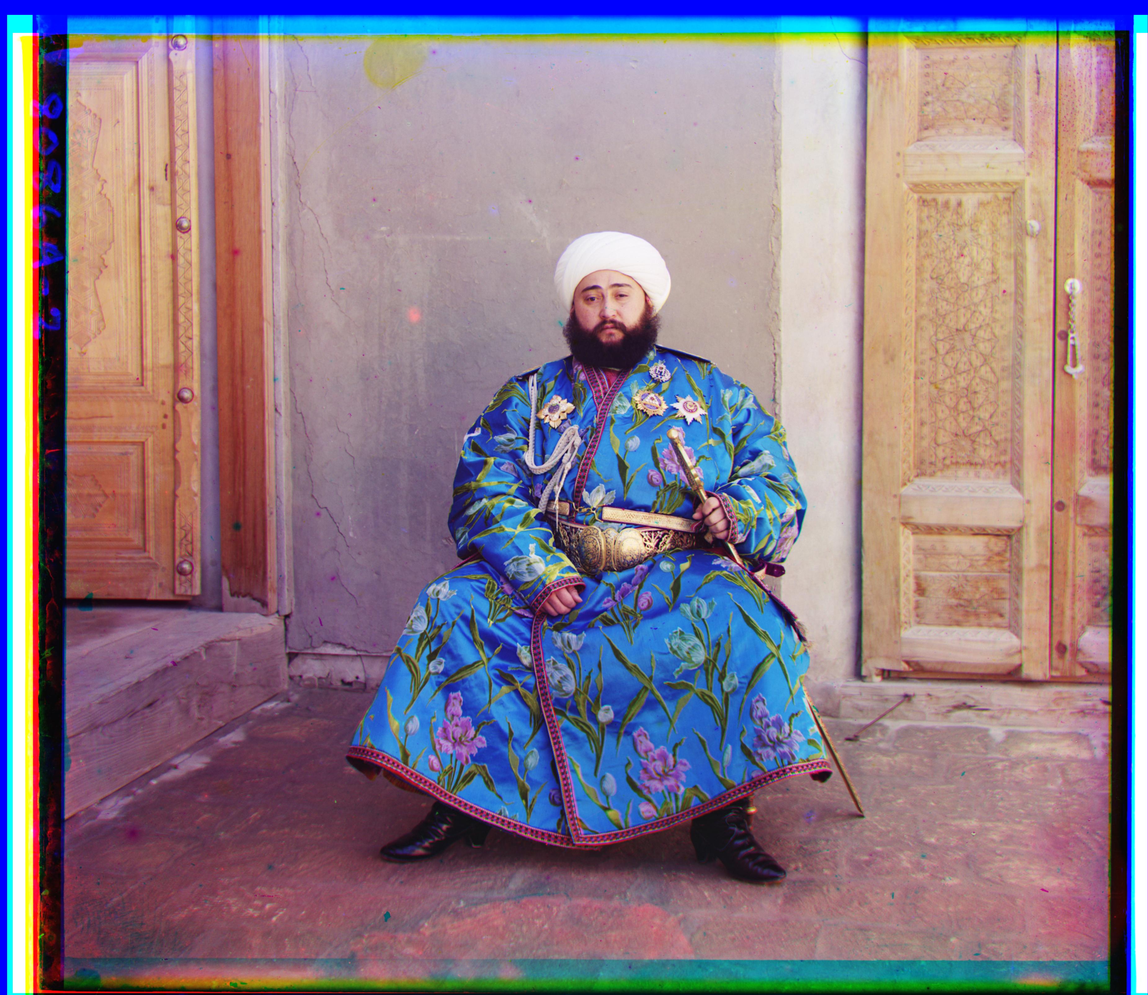
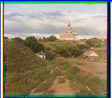
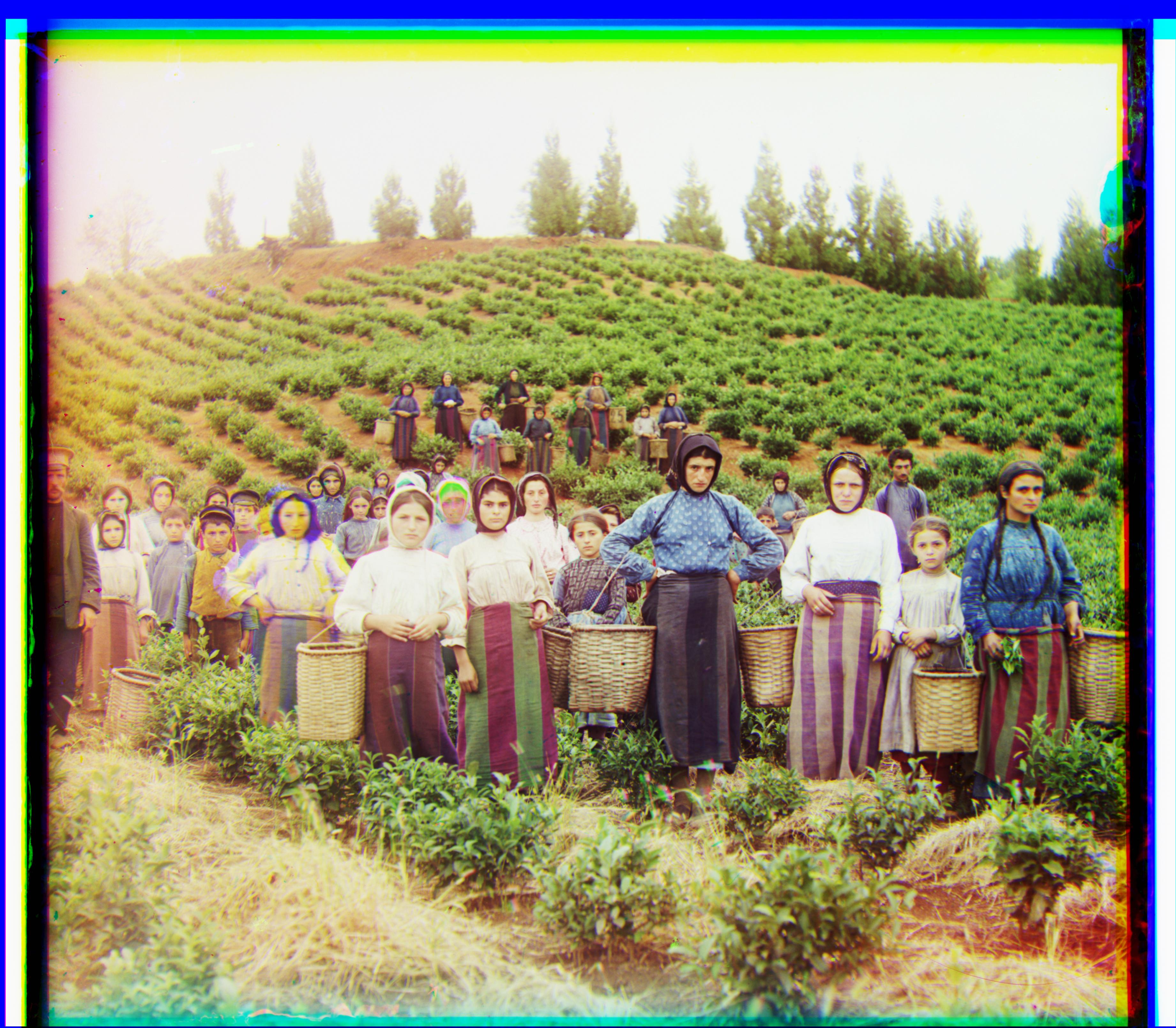
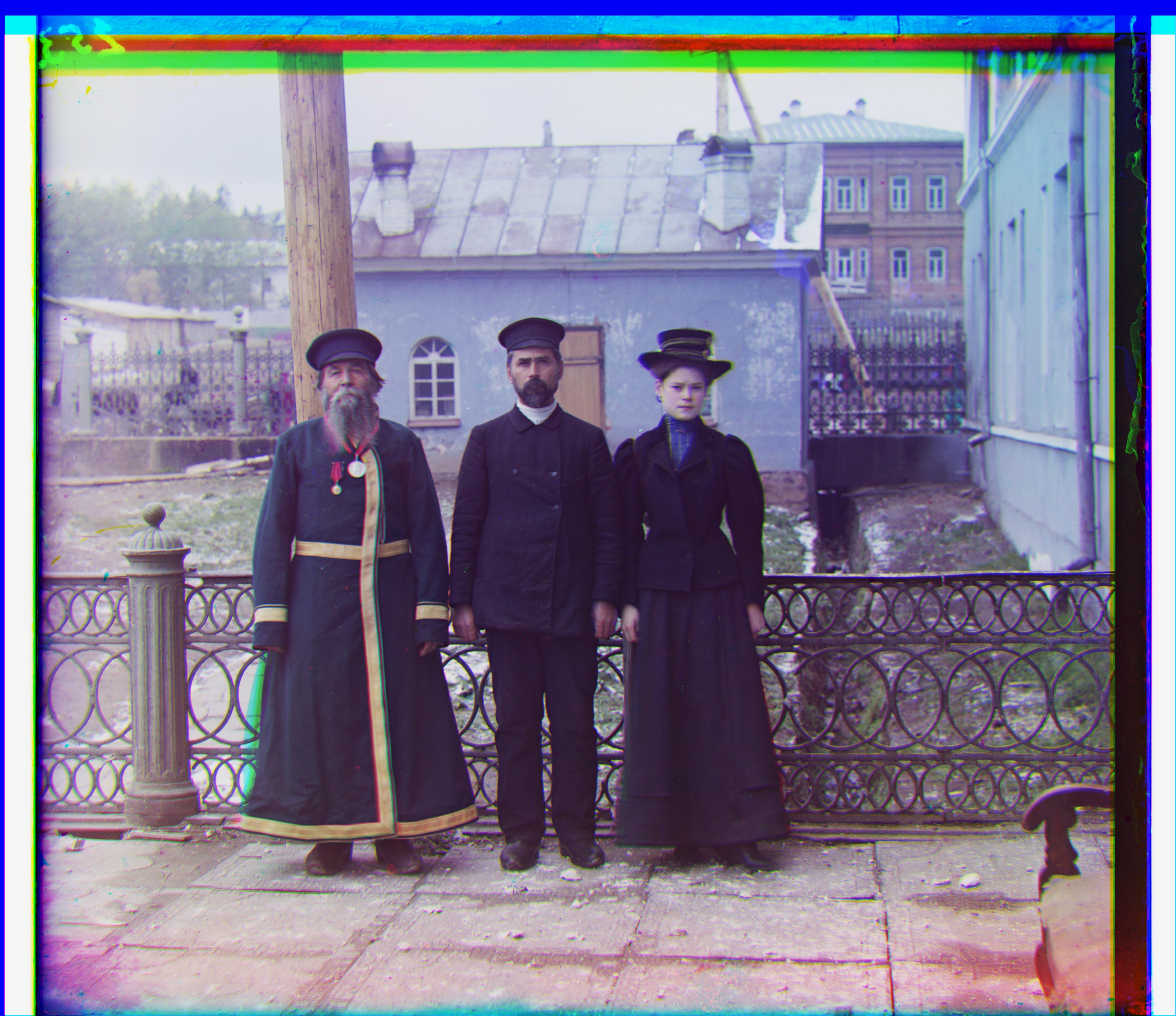
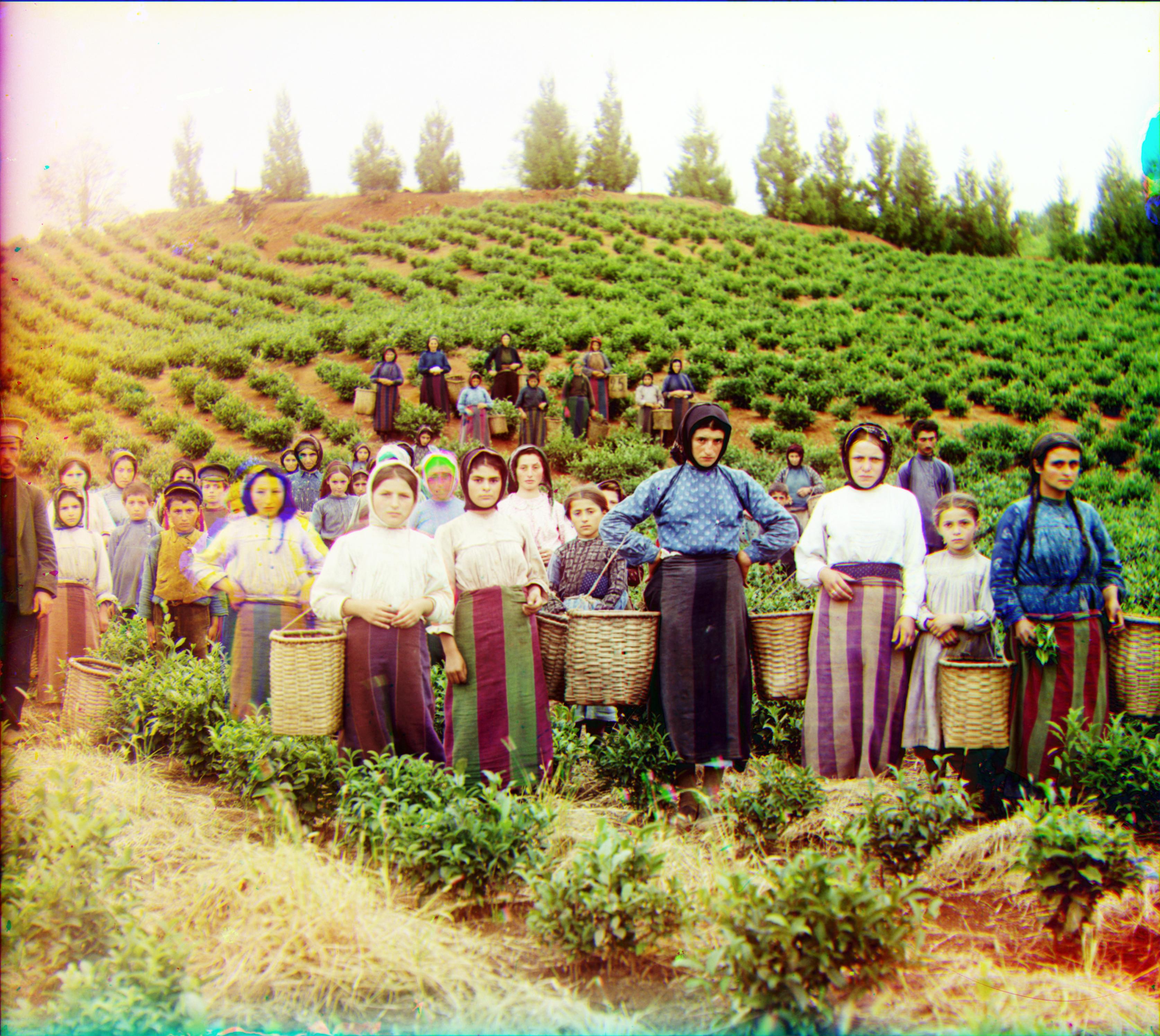
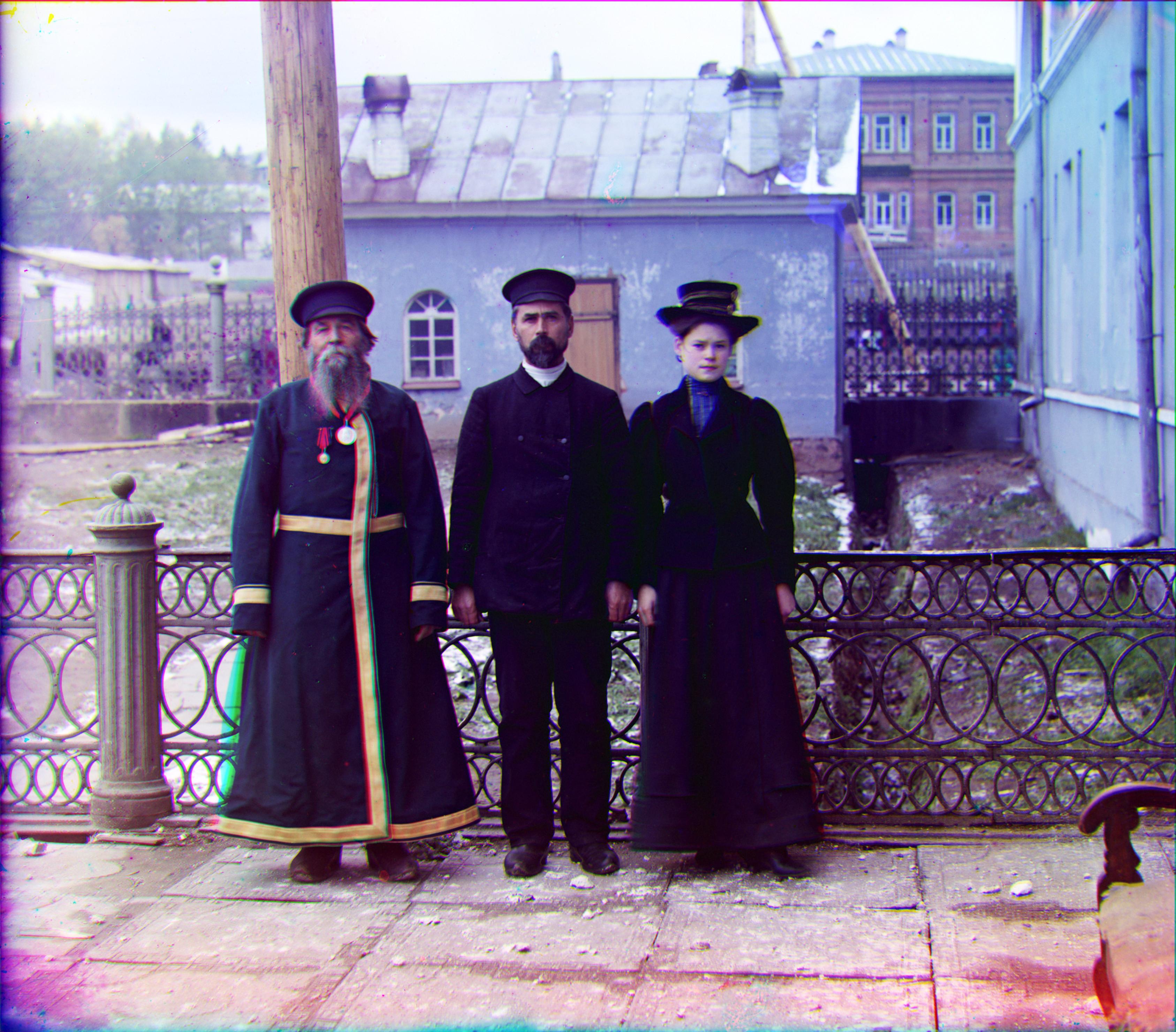
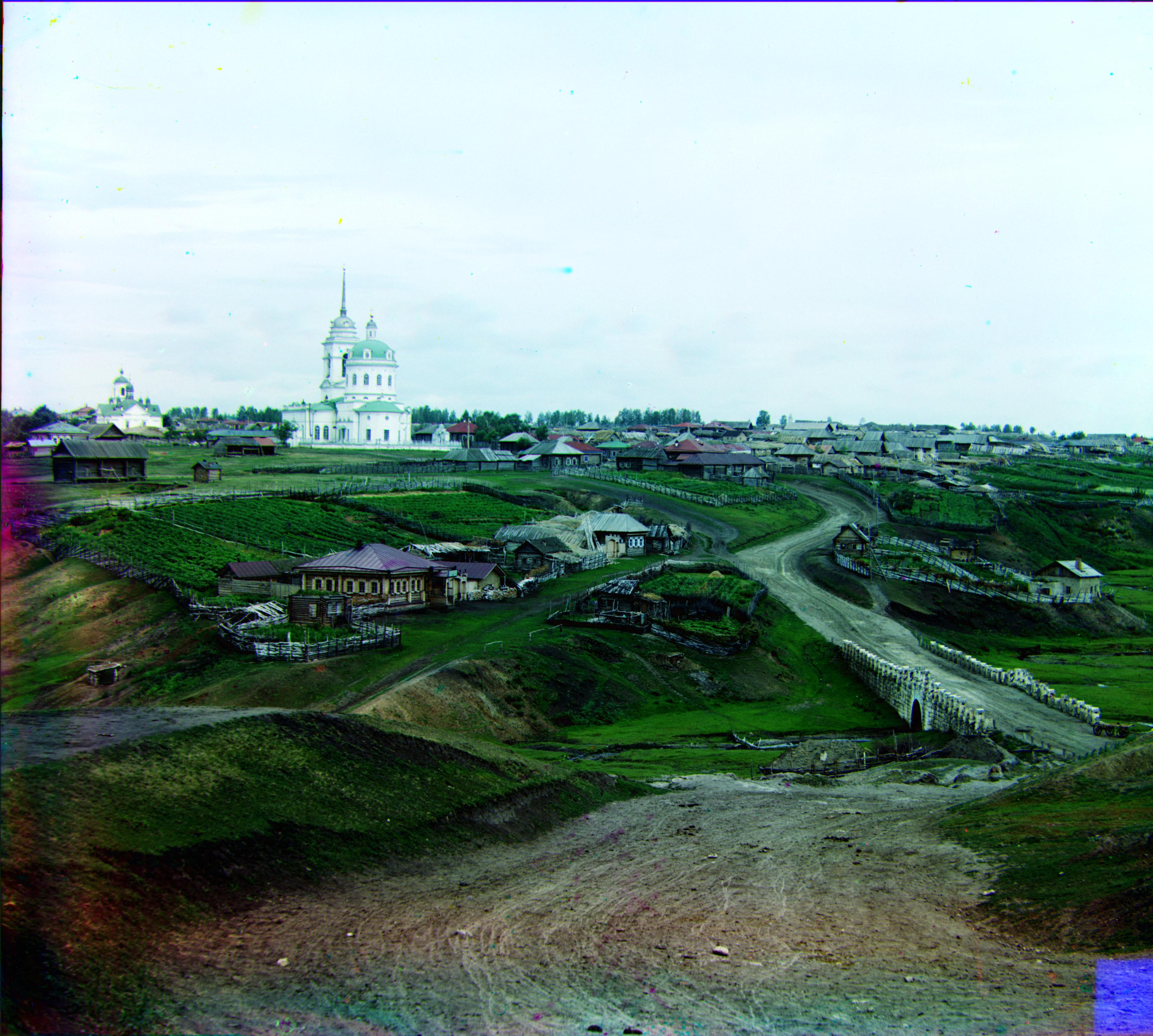
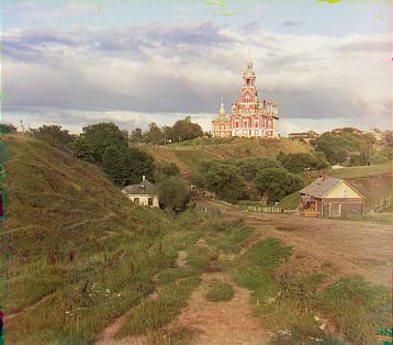
Please find the results for the remaining images below.

r_shift: (23, 136), g_shift: (13, 64)

For what it's worth, I implemented all of the above with only the allowed libraries for the non-bw section. I did this because this was originally going to be my non-bw submission. However, I opted not to because the runtime was a little slower than using NCC.

Automatic Border Cropping

One aspect of these merged images that has been troubling me is the is the border. Not only does it not look nice, but it added difficulty in section Image Pyramid NCC and I had to modify my code to accomodate it. I thought it would be best to devise a way to automatically remove the border.

As a first step I gaussian smooth the image. This is because I want to remove high frequency content. The border will later be detected as an edge, and I do not want any spurious high frequency areas misrepresenting a border. With much experimentation, I settled with a σ as 2 for gausssian blurring.

Next, I calculate the gradient of the image. However, this time I use a Sobel filter, Instead of the 1D gradient filter that I used in BW Grad. I chose to use a Sobel filter because the edges appeared sharper. I then use the x and y gradients to calculate the gradient magnitudes and directions.

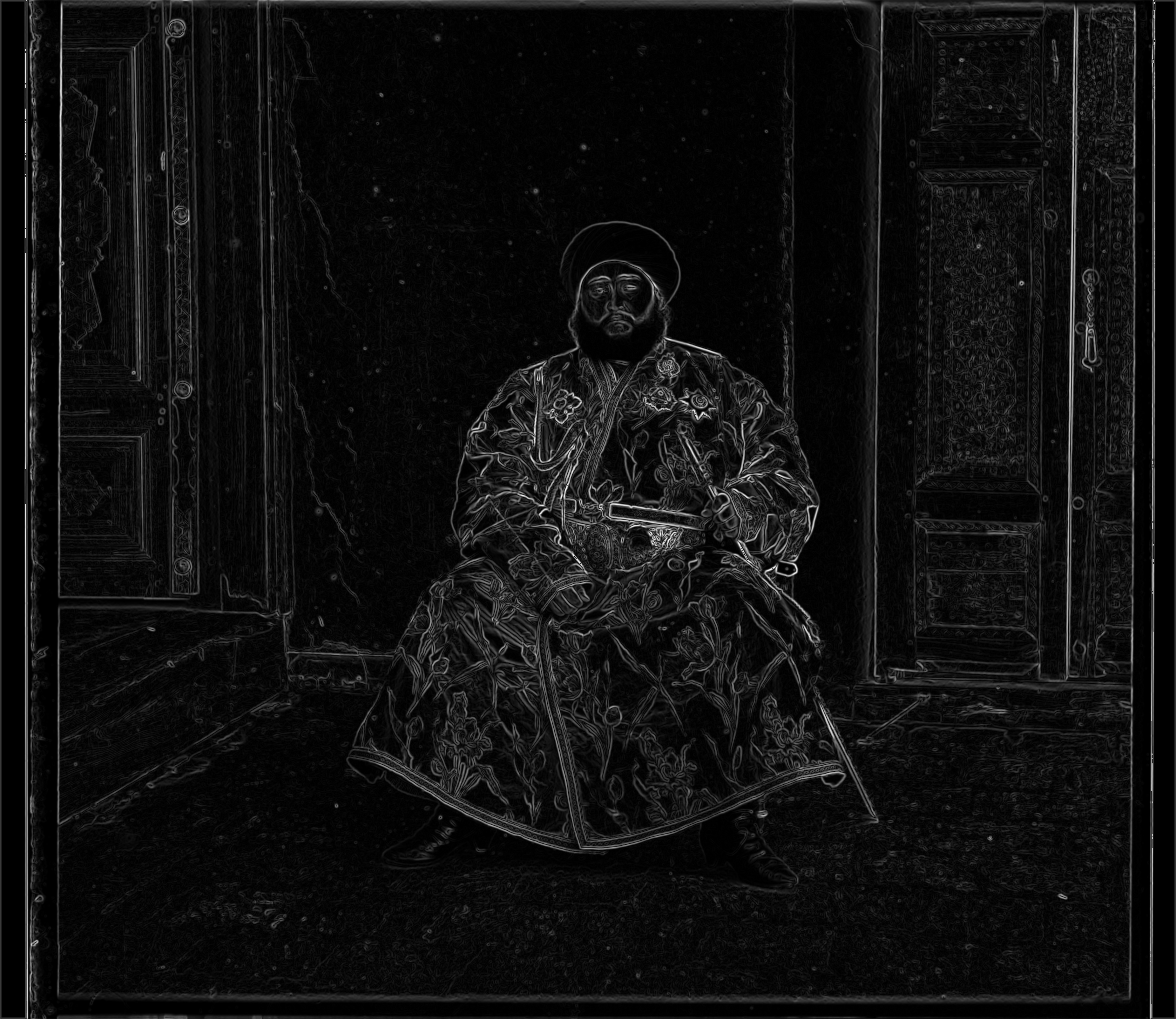
Borders will be areas in the image with strong edges in the vertical and horizontal directions. Therefore, I filter out all edges that are not vertical or horizontal, within a tolerance of ten degrees. I also filture out noisy gradients by removing those that are not within 1% of the maximum gradient magnitude. I then use all pixels with gradients remaining to create a mask.

Gradient Mask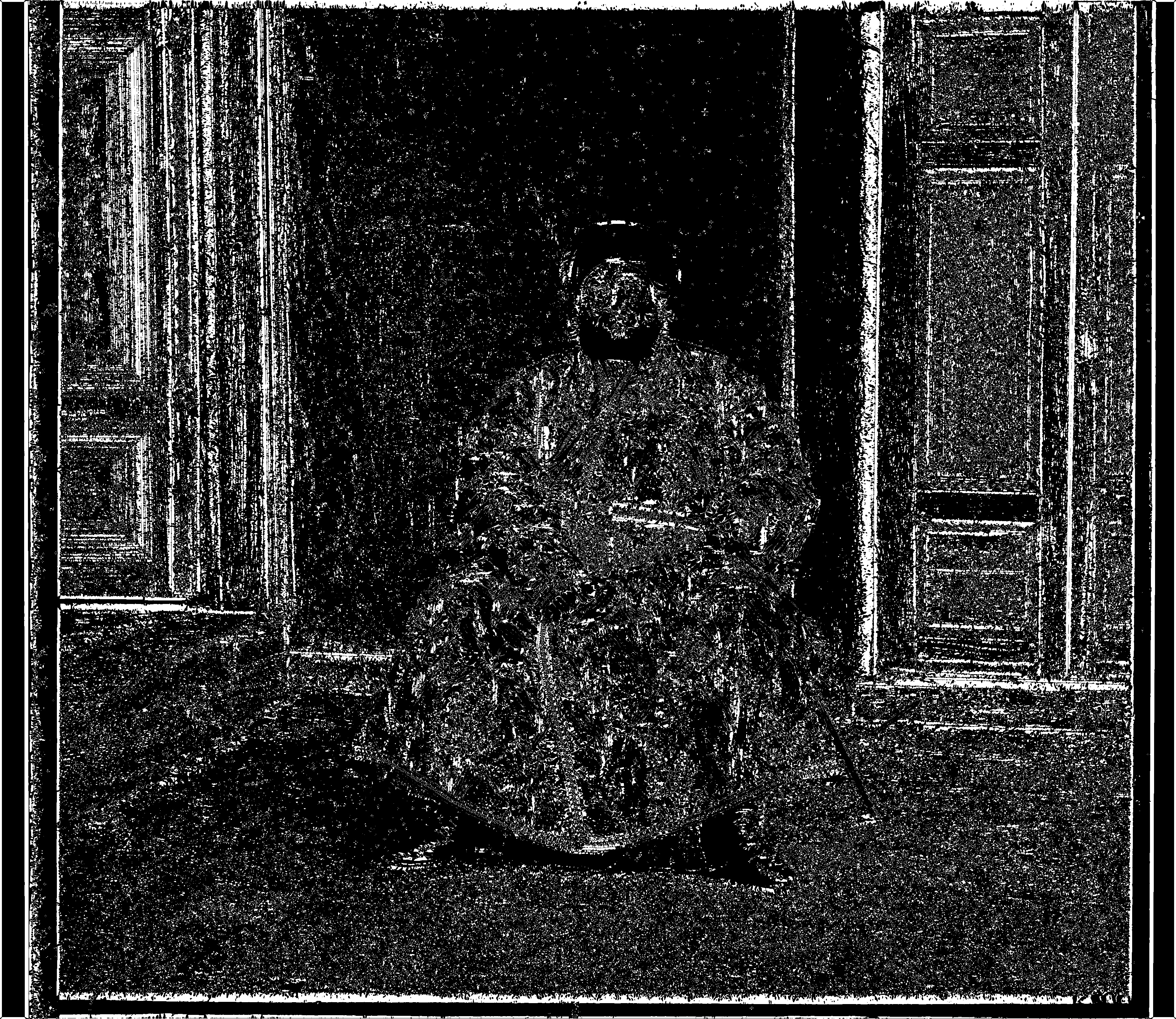

As one can see, while there still are gradient values scattered throughout the image, they predominantly lie on the vertical and horizontal lines.

To detect the vertical and horizontal lines in the image, I used the Hough Transform. How the Hough Transform works is it takes every mask point in the image and finds every line that the point could pass through. Lines are paramaterized into polar coordinates, ρ and θ, and each point provides a vote for all ρ and θ combinations that it could pass through. ρ and θ with enough votes are evalutated to be a line. My ρ and θ parameterizations where both 1. The toughest part was choosing the vote threshold to distinguish a line. Some channels in some images have additional vertical edges that were not borders that would sometimes be detected. Because of this, I kept the vote threshold higher to not detect these incorrect edges. However, this came at a cost of possibly missing some borders. This is resolved by both making this process iterative (as described below), and by running this process on all 3 channels. It is unlikely for the same border to be missed by all 3 channels, and after merging the images any part of one channel that fills into the border of another is cropped.

To crop the image, I use the borders of the innermost lines on all four sides. However, because my line threshold depends on the largest side of the image, it is possible some inner lines are not detected. To resolve this, I make the above process iterative until no new lines are detected.

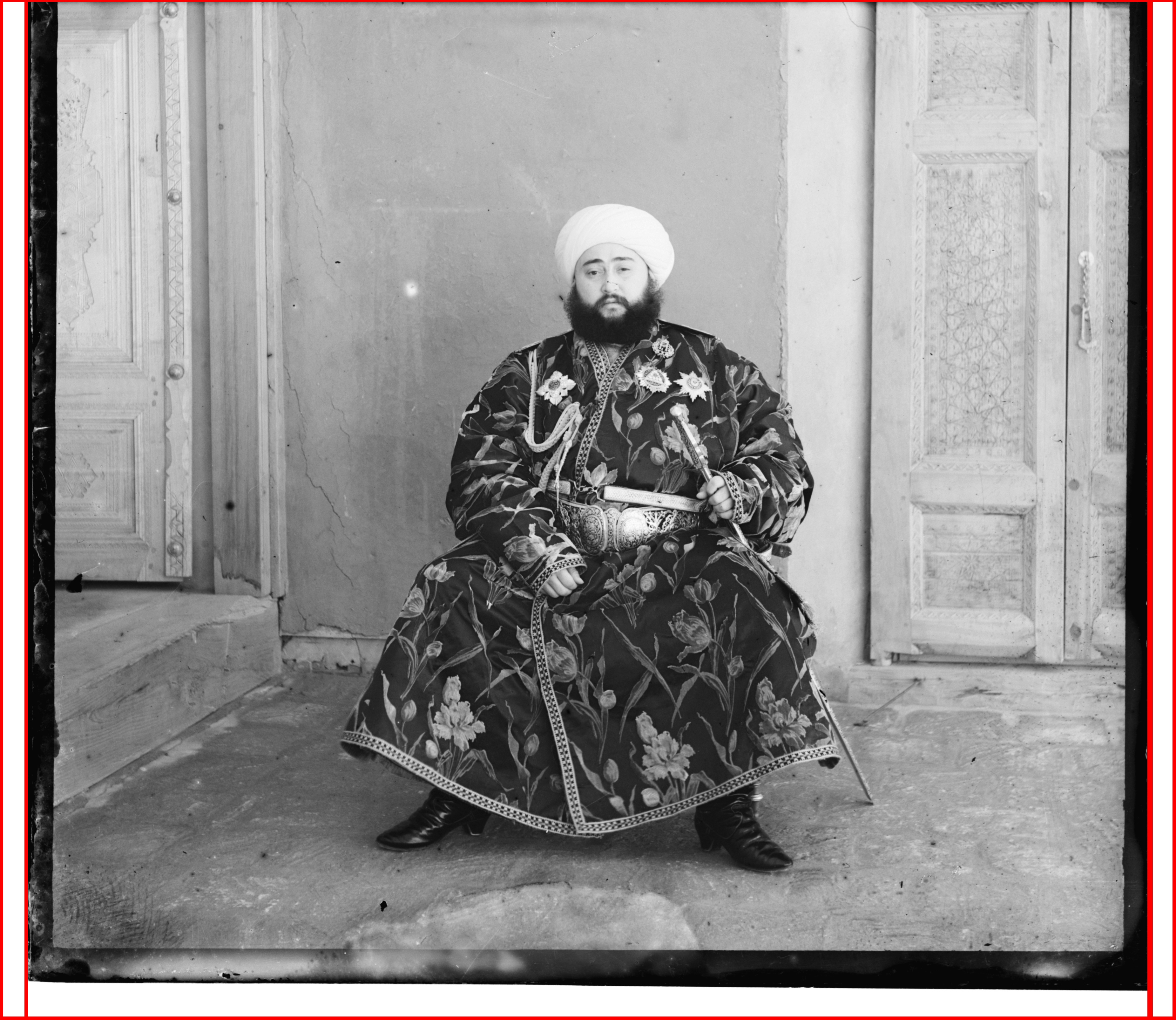
All of the above steps are run before finding the best translation. After the best translation is found, there is an additional cropping process where if any one channel's previously found border is in the new image, that area is cropped. The result is images whose borders are cropped. Notice even in the emir.tif case, the channel whose border was not fully detected was still found in at least another channel, and the border was cropped correctly.

Below are the results on the other images.

Automatic Contrasting

Next, I thought it would be fun to implement automatic contrasting. The assignment suggested "to rescale image intensities such that the darkest pixel is zero (on its darkest color channel) and the brightest pixel is 1 (on its brightest color channel)". To do this scaling, I first took the rgb from using BW Grad and BW Crop. Then, I made a cdf of all the pixel values. Because pixels may fall within a more meaningful range than [0, 255], I calculated the range of pixel values I wanted to use by trimming values off the cdf that were not within [1%, 99%].

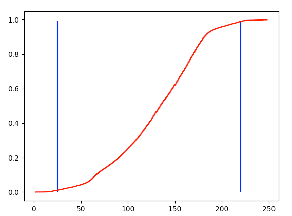
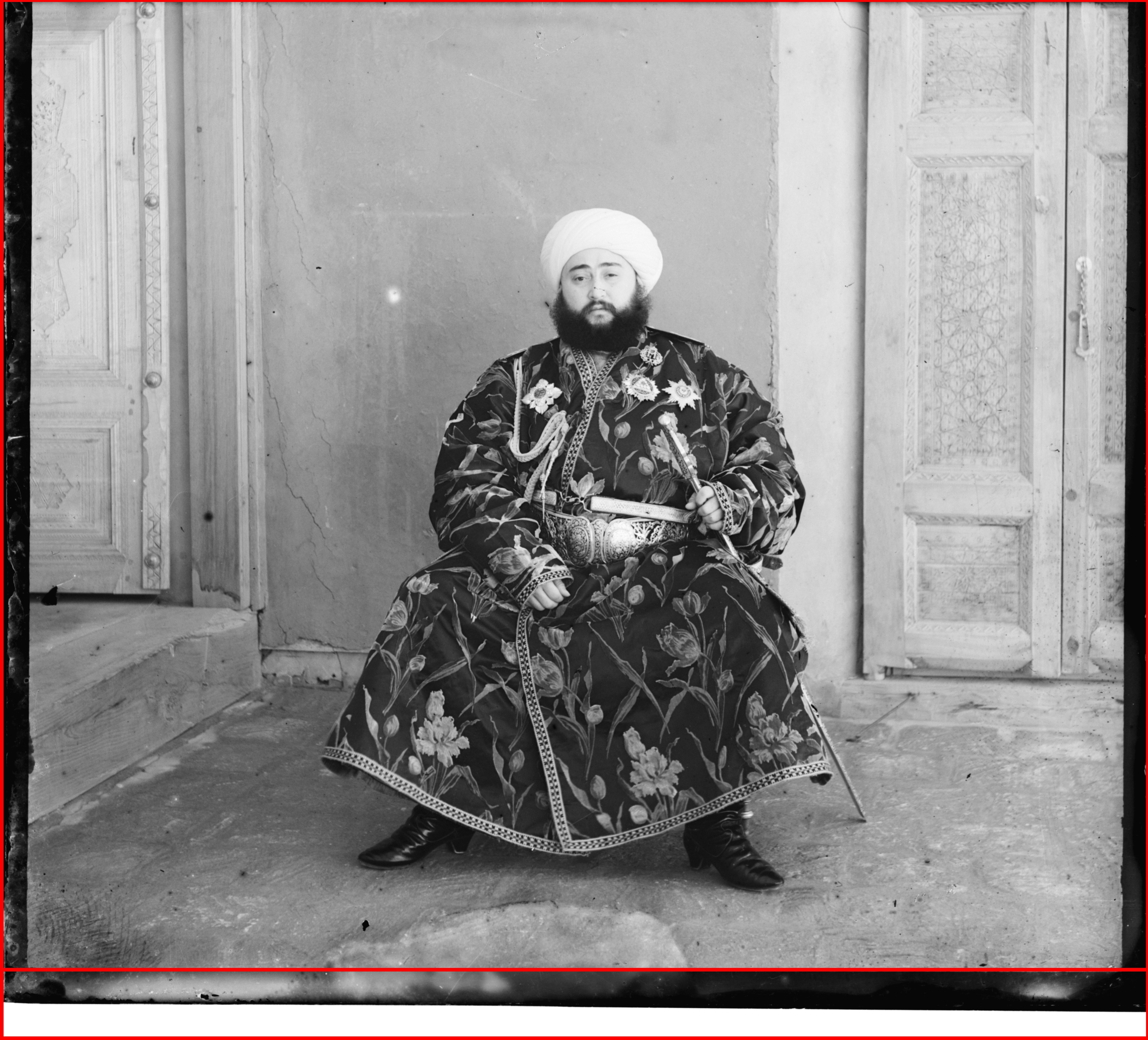
I then used the min and max pixel values in this range (corresponding to 41 and 223 in the example above) to calculate the alpha and beta values I would use to contrast the image. Alpha was caclulated as 255 / (max - min) and beta as -min * alpha. This way, the new pixel values in this window would fall within the range of [0, 255] when performed under the operation pixel_new = alpha*pixel_old + beta. I then scaled the rgb image to get the new image with better contrast. Notice how Emir's belt and robe are shinier and there is more noticable colour in the door.

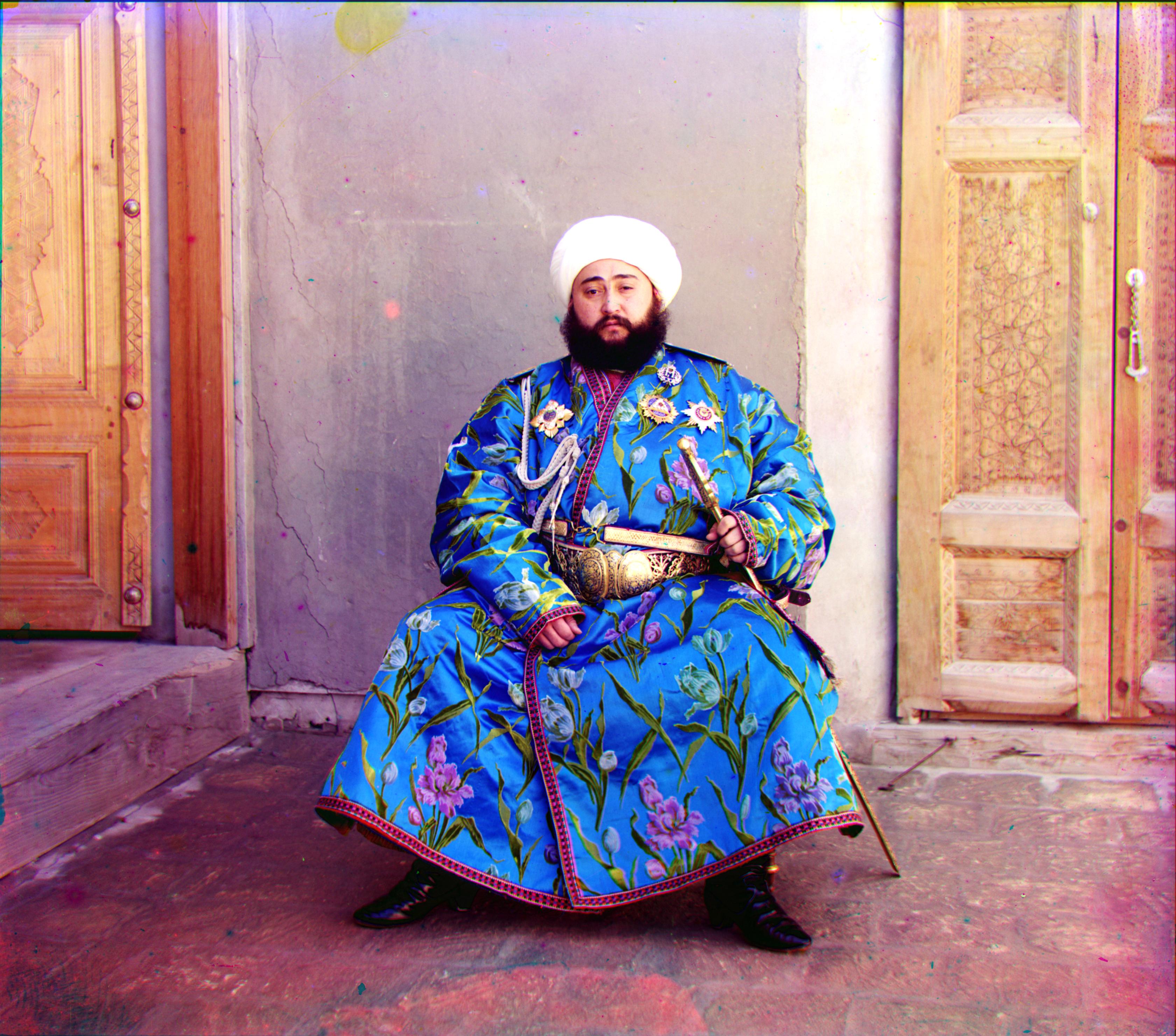
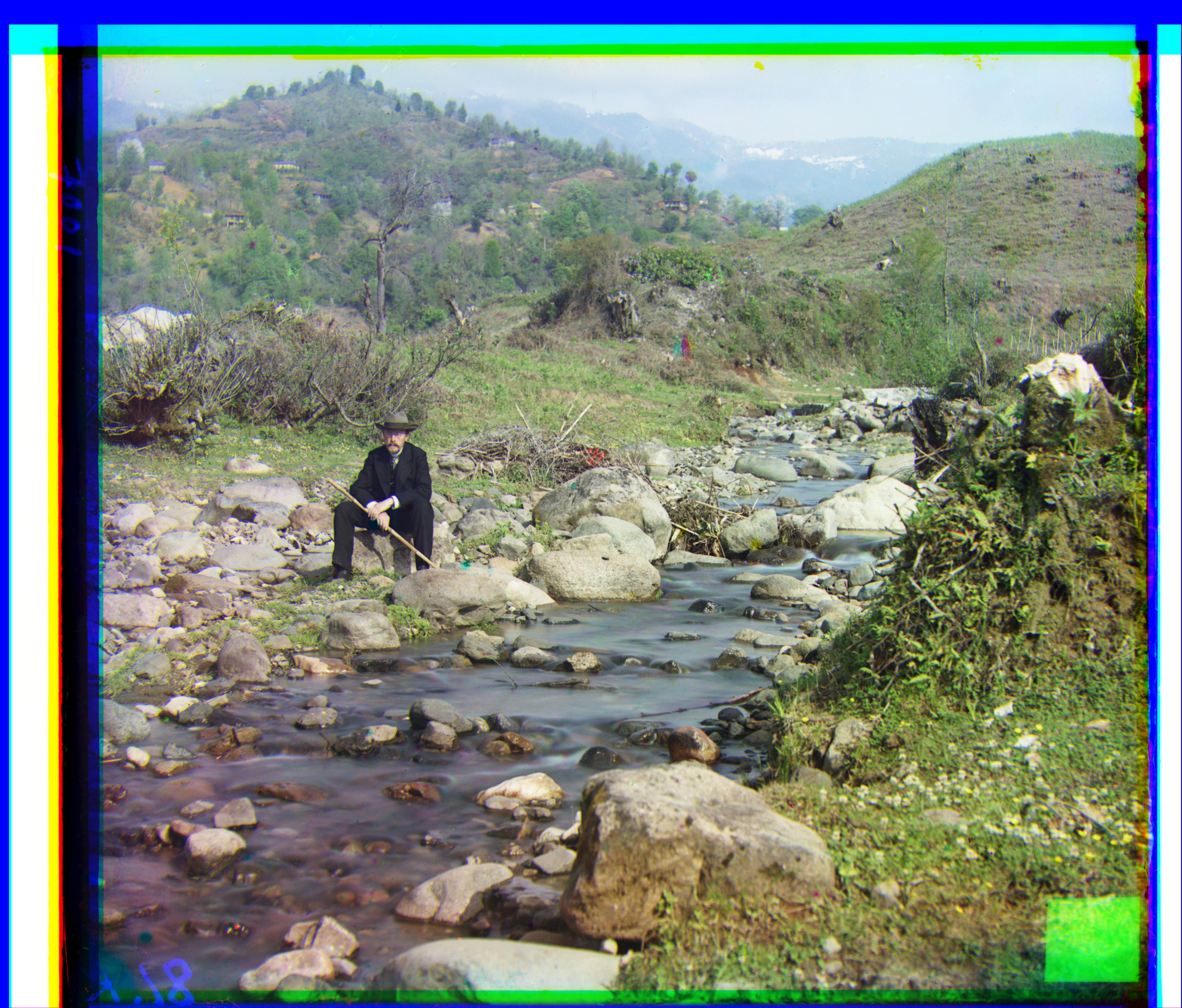
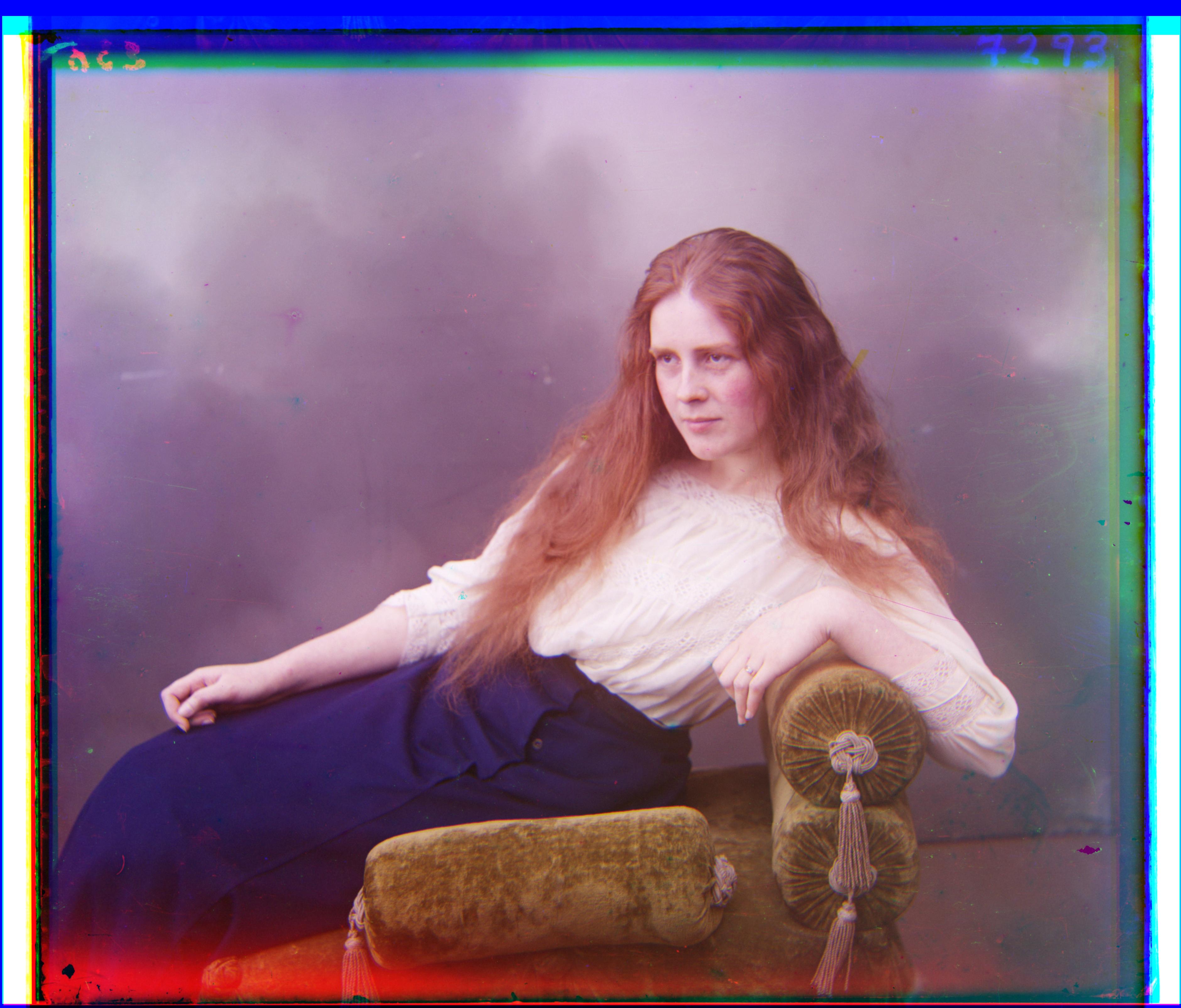
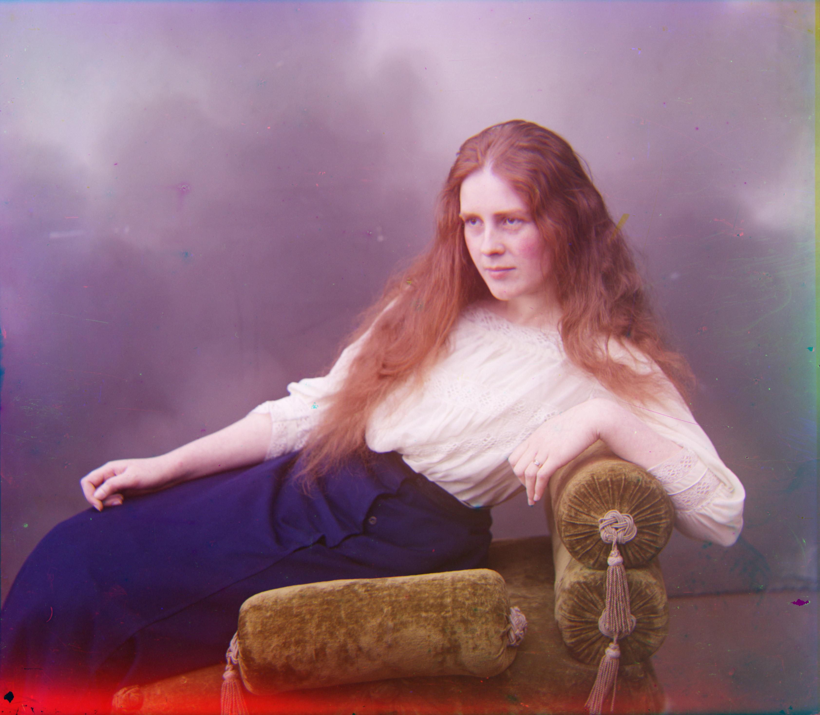
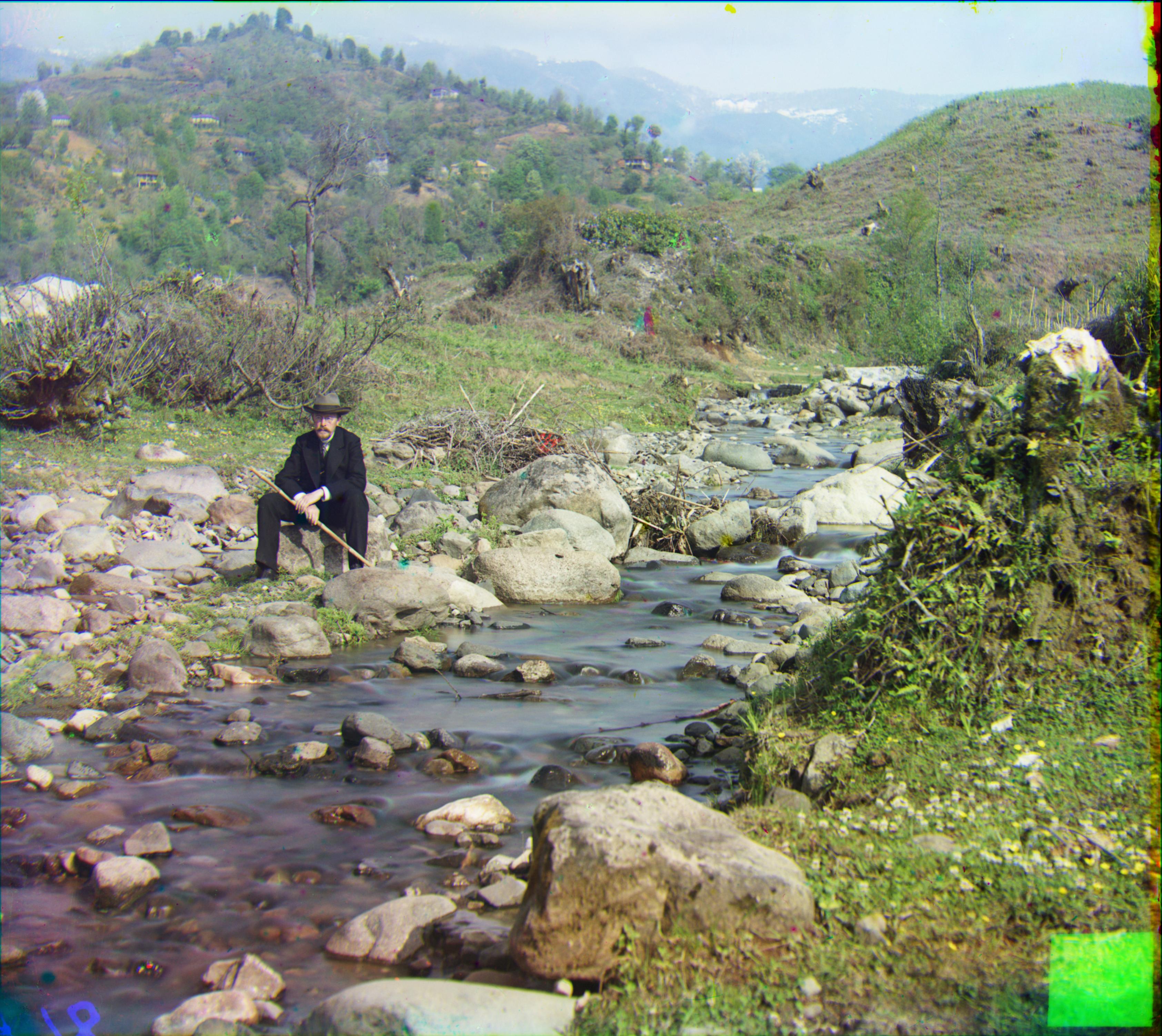
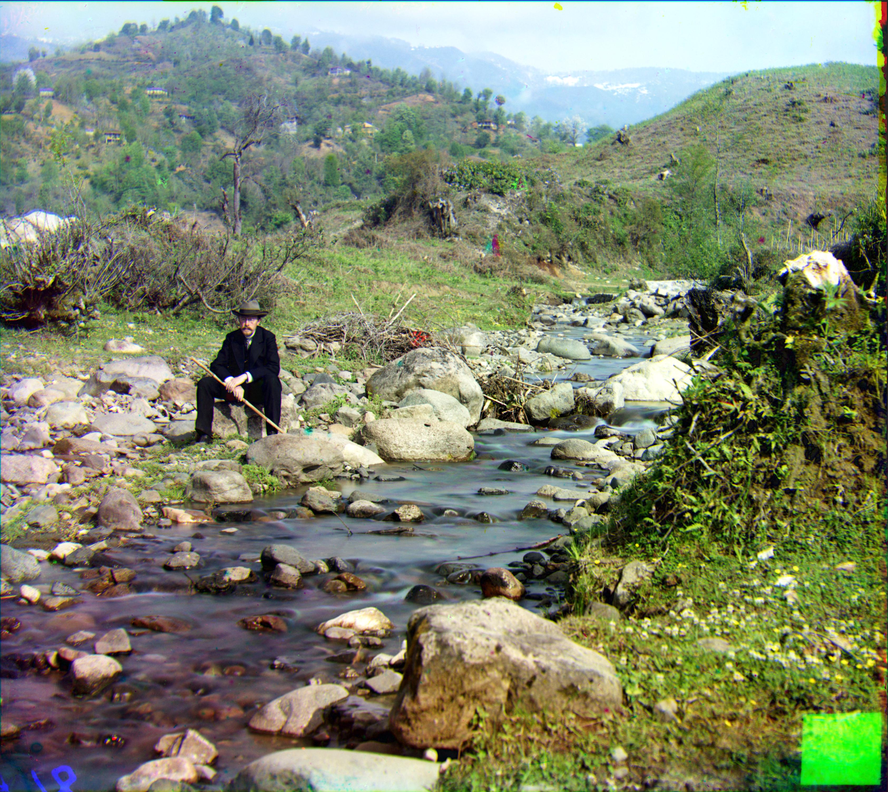
Below are the results on the other images. One of my favourites is the result after contrasting self_portait. The image looks much crisper.

Removing Blemishes (Attempt)

The final aspect that bothers me are the occasional colour blemishes, as seen in cathedral.jpg. There is a section of green on the left that stands out a little too much that I would like to try to resolve.

cathedral.tif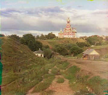

To do this, for each channel I find all pixel values that are 0 and use that to create a mask. I then find all the contours in the image using the open-cv findContours function. I filter the contours based on an area threshold to isolate the large blemishes.

Mask

I then define a border around the contour of size 20 pixels and find all pixels in this grid in the other two colour channels that do not fall in the contour area. I use these pixels to find the line of best find channel_contour = (channel_a - channel_b)*b + a where channel_contour is the channel we are operating on, channel_a and channel_b are the other two channels, and b and a are the line coefficients. I then use this line to approximate the pixel values in the contour area. The result is a blemish that is less noticeable. Here are an example.

Unfortunately, the image with the only noticeable diffence is cathedral.jpg. The blemish's in the other images are different in that there are colours that are not black. This makes the masking and finding the contours a little more difficult. If I had more time, this is something I would investigate more, and try to remove more complicated blemishes.