Click here for input/output files for Example 3
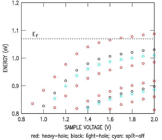
This example illustrates the occurrence of inversion. The bandgap is set to 1.17 eV bandgap, like that of Si, but since we still have a direct conduction band the simulation does not accurately reflect Si but rather it provides an estimation of inversion in Si. We examine low-doped n-type material with fairly large, positive voltages, such that the valence band edge at the surface crosses the Fermi-level and inversion could in principle result. (It should be noted that whether inversion actually occurs depends on the equilibrium of the carriers, as discussed in Phys. Rev. B 71, 125316 (2005) and also in N. D. Jäger et al., Phys. Rev. B 67, 165327 (2003)). The plot below shows the energies of the localized states in the valence band, plotting the results from FORT.30, FORT.40 and FORT.50.
Examining the results in the FORT.16 file, it can be seen that for the voltage points up until 0.8 V the self-consistency loop plays no role at all (exited after a few iterations) since the surface and bulk charge densities are essentially zero. A localized state does exist, but it's so far from the Fermi-level that it holds negligible charge. The output after each iteration shows the sample voltage (the "bias"), iteration number, band bending at point opposite the tip apex, number of localized states, and the surface and bulk charge densities (in cm^-2 and cm^-3, respectively). At a sample voltage of 0.9 V some nonzero charge is detected and the self-consistency loop is executed 15 times before exiting. Note that on the 6th iteration an apparent irregularity in the output occurs, with the charge densities appearing quite different than on the 5th or 7th iterations. This irregularity is due to the computation of the occupation of the localized states, which for the rather coarse number of energy steps used (200) is somewhat irregular. Increasing the number of energy steps to 2000 eliminates this problem.
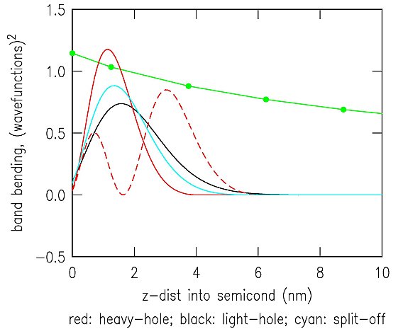
Wavefunctions can be examined in files FORT.31, FORT.41, and FORT.51. Shown below are the wavefunctions for sample bias of 1.2 V (and obtained by using an output parameter of 2 in FORT.9), together with the potential at the discrete grid points (shown by green dots). The wavefunctions are seen to have substantial magnitude over just a few grid points in the z-direction. If the results are examined at larger z-values, then the maximum limit over which the wavefunctions are computed is seen to be 66 nm. This values corresponds to the limit entered on line 44 of FORT.9, as also listed in the FORT.16 output file. In the radial direction, range over which the wavefunctions have substantial magnitude can be seen by inspection of the img1.PGM image (and is also listed in the FORT.16 output file), and they are similarly found to extend over just a few grid points.
It should be noted that this VERSION 6 of the program has not been thoroughly tested for all such inversion type situations. Problems involving overflow of the wavefunctions when integrating through a forbidden region could conceivably occur. Such problems can possibly be avoided by appropriate setting of the z-limit parameters on lines 49 and 54 of FORT.9, as discussed in Integration of Schrödinger's equation.