Integration of Schrödinger's Equation

The method used in solving for wavefunctions is by integration of the Schrödinger equation in 1-dimension, the same as used in early studies of tunneling resonances (Ref. 1) and elsewhere. This can be accomplished numerically for any potential (see Eq. 3 of Ref. 2). We define z=0 as being the surface, and take z>0 in the semiconductor. We take the potential to go to zero as z goes to infinity, and we denote the conduction band edge at large z as E_C and the valence band edge at large z as E_V. Extended states and localized states are considered separately. In the conduction band the former have energy above E_C, so at large z values they connect continuously to harmonically oscillating states, whereas the latter have energy below the band edge and go to zero at large z values. For the valence band, the extended states have energy below E_V and the localized states have energy above E_V.

For each energy value within the relevant range of energies, integration of the Schrödinger equation is performed. Integration of the wavefunctions starts in the vacuum, with a wavefunction value (unnormalized) and its derivative as given according to the exponential decay in the vacuum. The wavefunction is then integrated back to the surface, the surface is crossed (maintaining continuity of the wavefunctions and its derivative divided by the effective mass), and the integration continues all the way through the semiconductor. This procedure is well defined for any potential variation within the semiconductor, and a 2-band model is used to described the variation in character of the wavefunction within the semiconductor bandgap region. When the maximal value of z is reached (line 44 of FORT.9), the following procedure is employed:

For an extended state, it is analytically connected to a harmonic function of the type sqrt(2)sin(kz+θ) where θ is some phase angle (formally, this wavefunction would be multipied by a factor of 1/sqrt(L) where L is a normalization length, but that factor is cancelled when performing the sum over wavevector or energy). This connection then determines the magnitude of the wavefunction throughout the semiconductor and vacuum.
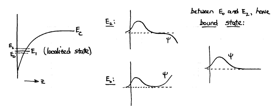
For a localized state, the integration through the forbidden energy region will never produce a wavefunction that goes perfectly to zero. Rather, the magnitude of the wavefunction will in general exponentially increase (albeit slowly), as illustrated in the diagram below. However, comparing results for one energy value compared to the next, this divergence will change in sign (i.e. a zero in the wavefunction will be formed). The formation of such a zero signifies a localized state, and the wavefunction up to the location of the zero can be taken as an estimate of the true wavefunction (with all wavefunction values set to zero beyond the location of the zero). For a fine enough spacing in energy, a very good estimate of the wavefunction and associated energy of the state is obtained. The localized state is then unit-normalized over its extent, thus determining the magnitude of the wavefunction throughout the semiconductor and vacuum. It should be noted that, according to this procedure, no matter range of z-value are considered in the problem the localized wavefunctions will always "fit" into this range, since by definition they go to zero at the end of the range. The user may ensure that a large enough z-range is used (line 44 of FORT.9) in order to obtain a realistic estimate of the wavefunctions.

For an inversion situation, the above prescription works fine. For VERSIONS 4.1 or 5.1 and above, we use only a single-band model (not a two-band model) in computing the decay length of the wavefunction for energies within the band gap. In other words, the inverse decay length increases monotonically as the energy between the state and the band edge increases. So, for conduction band (CB) inversion states as pictured below, their wavefunctions will decay uniformly as a function of distance into the semiconductor (even for very large distance such that the energy enters the allowed region of the valence band (VB)). Thus, the maximal z-range should be chosen to be sufficiently large, as described above, but it's fine if its value is very much larger than the minimum acceptable one.

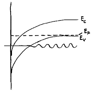
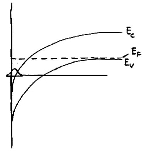The situation also works nicely for states of the CB, as shown below. Even with a very large maximal z-range, these states will be included in the computations but their magnitude will be very small since the states decay all the way up to the surface, and so no problem situations occur.

In VERSIONS 4.0 or 5.0, a two-band model was employed (see discussion near the end of the program documentation for VERSION 4 or VERSION 5). Then, as pictured below, integration of the Schrödinger equation results in CB states being analytically connected to VB state and vice versa. In that case, it was important to set the maximal z-range such that it cut off the integral in the middle of the band gap region.

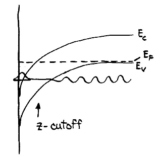If the value of the maximal z-range was too large, then the localized inversion states (CB states in this example) would extend into the VB and their amplitude would become somewhat ill-defined (due to an over-simplistic form used for the decay length in the two-band model, as well as because of the fact that, even with a better form, the effective masses in the two connected bands are equal within the model). Also, states from the CB would extend through the allowed region of the VB as they approached the surface, and again their amplitudes would be ill-defined. Moreover, a computation of inversion current in this case would include contributions from both the VB and CB, i.e. double counting the current. To avoid these problems it was necessary to precisely set the value of the maximal z-range for any given problem, and this procedure can be difficult for a non-expert user. For this reason, in VERSIONS 4.1 and 5.1, only a single-band model is used for computing the decay length of the wavefunction. This change was accomplished simply by commenting out the relevant lines of the code, as described in the program documentation for VERSION 4 or VERSION 5. If one wants to test out the effects of the two-band model (which is a better description than a single-band model), then one can restore the those lines, so long as, for inversion situations, care is taken to set an appropriate value for the maximal z-range (line 44 of FORT.9) in accordance with the diagram above.

References:
1. R. S. Becker, J. A. Golovchenko, and B. S. Swartzentruber, Phys. Rev. Lett. 55, 987 (1985).
2. R. M. Feenstra, Y. Dong, M. P. Semtsiv, and W. T. Masselink, Influence of Tip-induced Band Bending on Tunneling Spectra of Semiconductor Surfaces, Nanotechnology 18, 044015 (2007). For preprint, see http://www.cmu.edu/physics/stm/publ/74/.