Computation of Tunnel Current for Bulk States (including consideration of image potential and field-emission resonances)

The computation of tunnel current for bulk states in the SEMITIP package follows the method described in Refs. 1 and 2. In Ref. 2, the Tersoff and Hamann approximation (Ref. 3) is employed in order to obtain the tunnel current from a specific region of the sample surface, i.e. as appropriate for a sharp probe tip. However, the manner in which this approximation was implemented in the theory (i.e. Eq. (A8) of Ref. 2) was a bit ad hoc. Thus, a more rigorous derivation was developed in Ref. 4. It is that method which is used to obtain tunnel currents in the latest version of SEMITIP (intcurr.f routine).

In all of the methods discussed in Refs. 1, 2, and 4, the wavefunctions used within SEMITIP are only envelope functions of an effective-mass state for the corresponding band. For tip states, that description is totally fine if we consider the tip to be a free-electron metal. But for the sample, taken to be a semiconductor, the use of envelope-function-only wavefunctions, and connecting those across the sample surface to free-electron wavefunctions in the vacuum, is a significant approximation. This is the essential approximation for all of the computations of tunnel current made with SEMITIP.

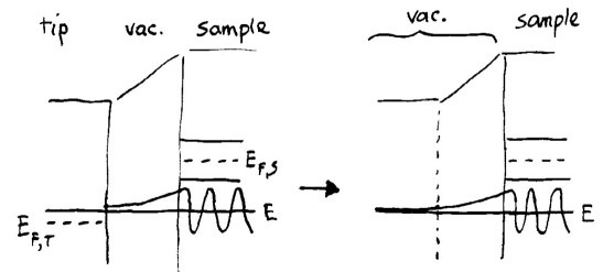
The method for computing tunnel currents used in Refs. 3 and 4, i.e. the Tersoff and Hamann approximation, treats the sample and tip quite asymmetrically. A computation is made of the sample wavefunction at the location of the probe-tip apex, with the spectrum of states for the tip not explicitly entering the theory. It is necessary to extend the results of Tersoff and Hamann to finite, possibly large, voltages. We accomplish that as shown in the diagram below, where the left-hand side shows the semiconductor bands of the sample and a particular state extending through the vacuum to the tip apex. Computationally, we start from the point on the tip apex and integrate Schrödinger's equation back through the vacuum and semiconductor, as described in Integration of Schrödinger's Equation. At the starting point, the derivative of the wavefunction is taken to be that corresponding to a simple exponential decay, i.e. the wavefunction itself times a decay constant, where the decay constant is √(2 m ΔE / ℏ²) where ΔE is the barrier height at the starting point. This value for the derivative corresponds to the situation for the sample states shown on the right-hand side where, in effect, we have replaced the tip by additional vacuum having a constant potential (corresponding to the vacuum level of the tip).

FIG 1. Schematic band diagram for tip and sample, showing a sample state extending through the vacuum to the tip apex. Evaluation of the state right at the tip apex is made as if the state there is purely exponentially decaying, i.e. as if the potential for the sample state in the absence of the tip is a constant from that point and further away from the sample. Band bending will in general occur within the semiconducting sample, but it is not pictured in this shematic view nor in the other diagrams below.

Let us consider a larger, negative applied bias between sample and tip. In that case the energy of a given state (the perpendicular component of the energy actually) can intersect the potential in the vacuum, as shown in the left-hand diagram below. If we take this situation literally, then we would have to construct freely-propagating sample states in the region where the energy is larger than the potential (i.e. a negative barrier). Forming those states by integration of Schrodinger's equation is no problem, of course, but such states cannot be well incorporated into the Bardeen formalism (which assumes only weak, tunneling states for the sample wavefunctions on the right-hand side on the barrier region), and neither do they fit will into the Tersoff and Hamann formalism (since it is based on the Bardeen formalism). Nevertheless, it is convenient for us to have some method to approximately handle this situation, just so that our computations can be extended slightly into this large, negative voltage regime. We choose to treat this situation by again extending the potential as a constant, but now starting from the intersection point between the energy of the state and the potential in the vacuum, as shown on the right-hand side below. The result of this extension is that the wavefunction is simply a constant for all spatial locations between the tip apex and the location where the energy of the state intersects the potential.

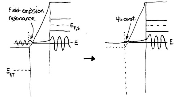
FIG 2. Schematic band diagram for a large negative sample-tip bias voltage. In this case the energy of the sample state intersects the potential in the vacuum. For extension of the sample states into this negative-barrier region, an approximation is made in which the wavefunction is a constant, i.e. as if the potential is extended as a constant from that point and beyond.

This extension shown on the right-hand diagram is clearly an approximation; as just mentioned it is designed to permit numerical evaluations out to slightly higher voltages than otherwise could be handled. In general, the computations of current using SEMITIP should be restricted to voltages with magnitude less than about 4 V, so that the barrier in the vacuum is everywhere positive (i.e. energy lower than the potential). Clearly, the occurrence of field-emission resonances at the tip cannot be treated at all in these computations.

Let us now consider application of large, positive voltages between the sample and the tip, as pictured below.

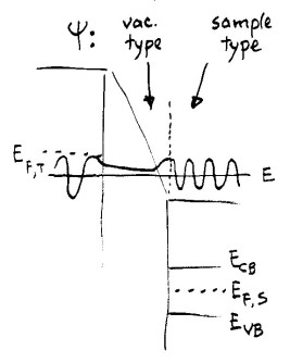
FIG 3. Schematic band diagram for a large positive sample-tip voltage, for which field-emission resonances occur in at the sample-side of the vacuum region where the energy of the state is higher than the potential in the vacuum (i.e. a negative-barrier). The wavefunction in this region is taken to be the vacuum type (i.e. with effective mass equal to the free-electron mass and energy measured relative to the potential value in the vacuum), the same as it is elsewhere throughout the vacuum.

In this situation, field-emission resonances of the sample will occur, and these can be treated, at least approximately, in the computations (i.e. with the extension of the sample wavefunctions into the region of the tip handled in exactly the same manner as in Fig. 1). However, it should be noted that our framework in which the wavefunctions are connected across the sample surface (i.e. using continuity of the wavefunctions and of the derivative divided by the effective mass) still applies. Hence the wavefunction when integrated through the vacuum region where the potential is less than the energy is a vacuum-type state, whereas when the wavefunction crosses the sample surface it is transformed into one of the sample-type states.

This matching process of the wavefunctions across the sample surface becomes considerably more problematic if an image potential at the sample surface is included, e.g. for small sample-tip voltages as shown in the sketch below.

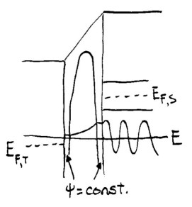
FIG 4. Schematic band diagram when an image potential is included in the vacuum. Now, the wavefunctions on the two extreme sides of the vacuum are treated as if the states of the sample and tip extend out slightly into the vacuum. This approximate treatement is accompished simply by taking the wavefunctions to be a constant in these regions where the energy of the state exceeds the potential in the vacuum.

In this sketch, we have included an image potential on both the sample and the tip side of the vacuum. However, it should be noted that within the Tersoff and Hamann approximation we are dealing only with states of the sample. In this sense our treatment is somewhat "mixed" and approximate, but it nevertheless serves to provide a useful upper bound on the effect of image potentials on the tunnel current. For intcurr version 6.2 and above, the possibility of including the image potential is included, and when that option is selected then the approximate image potential term from Eq. (33) of Simmons (Ref. 5), divided by two (Ref. 6), is added to the potential in the vacuum. At both the sample- and the tip-side of the vacuum, there is a small region where the energy of the state is larger than the potential in the vacuum. For the tip-side, we can deal with this situation precisely as shown in Fig. 2, i.e. by extending the wavefunction as a constant through that region. With this treatment, we are in a sense shifting the tip apex into the vacuum slightly, in accordance to how the tip states extend into the vacuum due to the image potential. How do we treat the situation on the sample-side of the vacuum? Now, it is not at all clear where the transition in the wavefunctions between "sample type" and "vacuum type" should be made; if we treat the states the same as in Fig. 3 then this transition would be made at the sample surface, but in that case we end up with a small negative-barrier region near the sample surface where the vacuum-type states have an attractive potential, which does not seem to be physically reasonable. A much more reasonable picture for the effect of the image potential is that the sample states themselves extend out slightly from the sample, in accordance to the image potential. To model that situation, we employ an approximation similar to that of Fig. 2, in which the wavefunction is taken to be a constant in this region where the energy is greater than the potential, as indicated in Fig. 4. Thus, we treat the wavefunction on both extreme sides of the barrier in the same manner. With this treatment, we no longer achieve any sort of description of the field-emission states of the samples, i.e. Fig. 3 no longer applies, since when the image potential is included then the wavefunction is assumed to be constant over the entire barrier region where the energy of the state is greater than the potential. But, loss of that description is of no great significance, since achieving it was not our aim to begin with. Rather, our goal is to describe the low-voltage spectroscopy, and with inclusion of this option of describing the image potential we have achieved an approximate description of its influence on the low-voltage spectra.

When the image potential is included in the computations, we find that the tunnel current increases by about three order-of-magnitude, with the magnitude of this increase being nearly independent of voltage. This result is consistent with our expectations for the influence of an image potential, as described in Refs. 1, 2 and 4.

References:
1. R. M. Feenstra, Y. Dong, M. P. Semtsiv, and W. T. Masselink, Influence of Tip-induced Band Bending on Tunneling Spectra of Semiconductor Surfaces, Nanotechnology 18, 044015 (2007). For preprint, see http://www.cmu.edu/physics/stm/publ/74/.
2. Y. Dong, R. M. Feenstra, M. P. Semtsiv and W. T. Masselink, Band Offsets of InGaP/GaAs Heterojunctions by Scanning Tunneling Spectroscopy, J. Appl. Phys. 103, 073704 (2008). For preprint, see http://www.cmu.edu/physics/stm/publ/79/.
3. J. Tersoff and D. R. Hamann, Phys. Rev. B 31, 805 (1985).
4. S. Gaan, G. He, R. M. Feenstra, J. Walker, and E. Towe, Size, shape, composition, and electronic properties of InAs/GaAs quantum dots by scanning tunneling microscopy and spectroscopy, J. Appl. Phys. 108, 114315 (2010). For preprint, see http://www.cmu.edu/physics/stm/publ/93/.
5. J. G. Simmons, J. Appl. Phys. 34, 1793 (1963).
6. J. G. Simmons, J. Appl. Phys. 35, 2472 (1964).