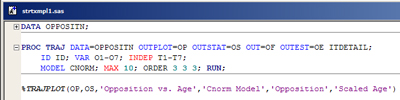
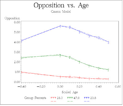
Example (SAS program strtxmpl1.sas): using start values to adjust group trajectories. This example shows how to create starting values to make adjustments to a trajectory model.
We'll use opposition behavior data (scale - 0 to 10) from the Montreal Longitudinal Study.
The strategy used here is to start with all cubic trajectories.
The order for each group is decreased so that the highest order parameter estimates (for trajectories beyond intercept only), are significant for each group.
Step 1: Fit the cubic trajectory model.
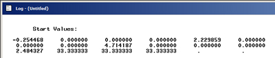
Three-group cubic trajectory model : The log shows the default start values.
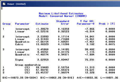
Three-group cubic trajectory model results.
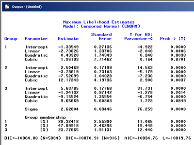
In group 1, the slope parameter is the highest significant term (p = 0.0406).
In group 2, the cubic parameter (p = 0.0037) is the highest significant term, while in group 3, the quadratic term (p < 0.00005) is the highest significant term.
So the appropriate orders are 1 3 2.
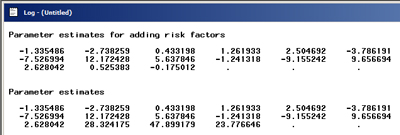
The log has the parameter estimate column from the output to ease cutting and pasting into the SAS program to create start values.
Parameter estimates are given in the log for cut and paste.
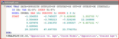
Step 2: Create start values from the first model results.
We're going to eliminate terms from the initial model.
The parameter estimates from the initial model are copied from the log.
Since this example does not use risk factors, the second set of parameter estimates are used.
Eliminated parameters have been commented out as shown below.
Modified three-group model with start values.
Final three-group model results.

SAS program: strtxmpl1.sas