SNA PhD 2025: Structural Equivalence

Author

Prof Brandy Aven

Published

November 19, 2025

Structural Equivalence in Social Network Analysis

This lab explores three different approaches to identifying structural equivalence in social networks: Euclidean Distance, CONCOR, and Optimization methods. Structural equivalence examines how actors occupy similar positions in a network based on their connection patterns.

Datasets

We’ll use two datasets for this analysis:

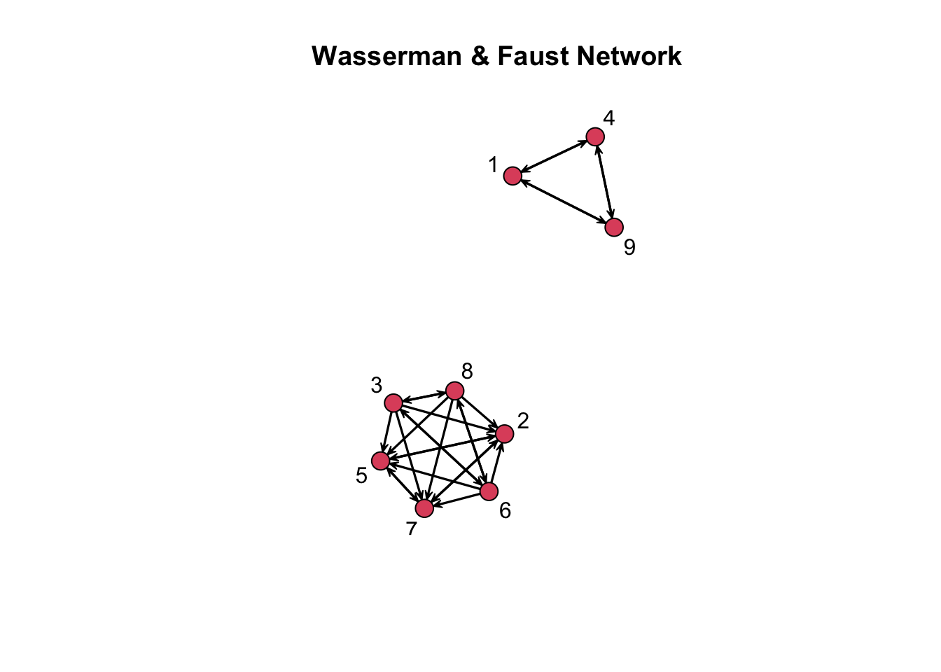
  1. Wasserman & Faust (1994) Network: A small network ideal for illustrating blockmodeling techniques

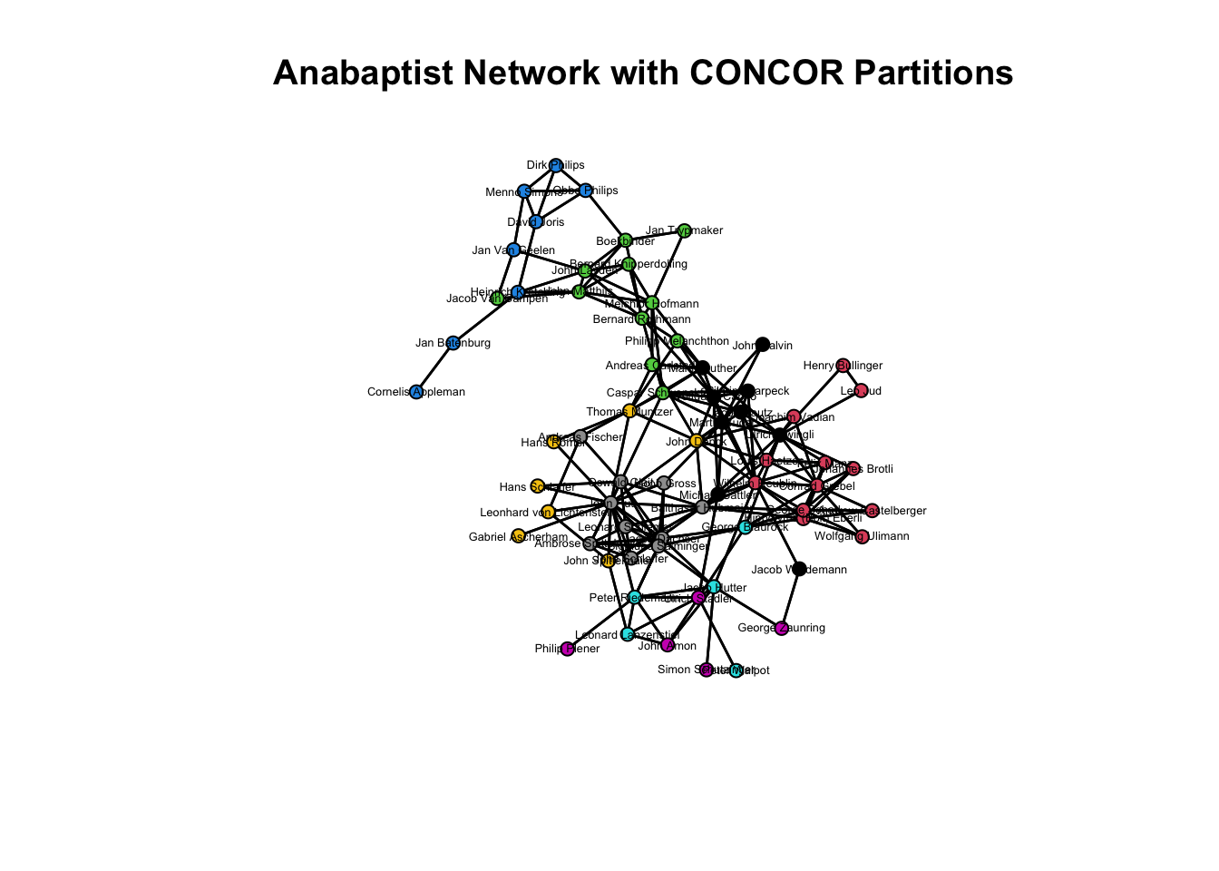
  2. Anabaptist Leadership Network: A larger network of 67 religious leaders during the Protestant Reformation

Import and Visualize Data Wasserman & Faust Data

Code
# Import Wasserman & Faust network
wfse.mat <- as.matrix(read.csv("WFSE.csv", header=TRUE, row.names=1, check.names=FALSE))
wfse.net <- as.network(wfse.mat, directed=TRUE)

# Display network summary
wfse.net
 Network attributes:
  vertices = 9 
  directed = TRUE 
  hyper = FALSE 
  loops = FALSE 
  multiple = FALSE 
  bipartite = FALSE 
  total edges= 27 
    missing edges= 0 
    non-missing edges= 27 

 Vertex attribute names: 
    vertex.names 

No edge attributes
Code
# Plot the network
gplot(wfse.net, usearrows=TRUE, arrowhead.cex=0.5, 
      label=network.vertex.names(wfse.net), 
      main="Wasserman & Faust Network")

Method 1: Euclidean Distance

Euclidean distance measures similarity by comparing distances between nodes in n-dimensional space. Unlike graph theoretical distance (path length), Euclidean distance represents the most direct route between actors.

Code
# Calculate structural equivalence using Euclidean distance
#wfse.eq <- equiv.clust(wfse.net, method="euclidean", mode="digraph")
wfse.eq <- sna::equiv.clust(
  wfse.net,
  equiv.fun = sna::sedist,      # force sna's sedist, not blockmodeling's
  method    = "euclidean",
  mode      = "digraph"
)


# Create blockmodel with 3 blocks
wfse.bl <- blockmodel(wfse.net, wfse.eq, k=3, mode="graph")

# Display block membership
wfse.bl$plabels
[1] "9" "1" "4" "7" "2" "5" "8" "3" "6"
Code
wfse.bl$block.membership
[1] 1 1 1 2 2 2 3 3 3
Code
# Show block model
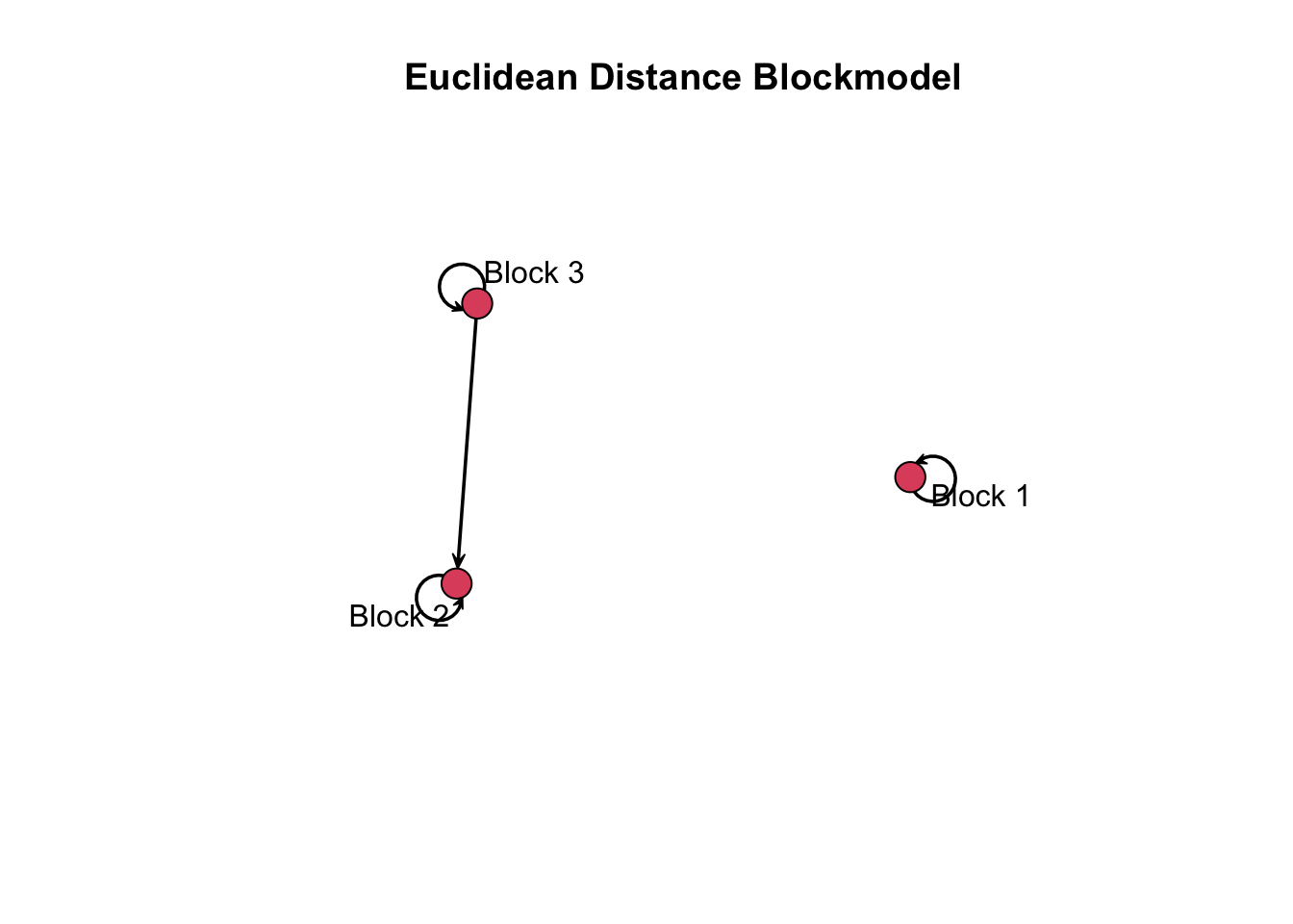
wfse.bl$block.model
        Block 1 Block 2 Block 3
Block 1       1       0       0
Block 2       0       1       0
Block 3       0       1       1
Code
wfse.bl

Network Blockmodel:

Block membership:

1 2 3 4 5 6 7 8 9 
1 2 3 1 2 3 2 3 1 

Reduced form blockmodel:

     1 2 3 4 5 6 7 8 9 
        Block 1 Block 2 Block 3
Block 1       1       0       0
Block 2       0       1       0
Block 3       0       1       1

Visualize Blockmodel

Code
# Convert to matrix and network object
wfse.blmat <- as.matrix(wfse.bl$block.model)
wfse.blnet <- as.network(wfse.bl$block.model)

# Plot blockmodel with loops
gplot(wfse.blmat, usearrows=TRUE, arrowhead.cex=0.5,
      label=network.vertex.names(wfse.blnet), 
      diag=TRUE, loop.cex=1.5,
      main="Euclidean Distance Blockmodel")

Distance Matrix

Code
# Calculate Euclidean distances
sna::sedist(wfse.net, method="euclidean", mode="digraph")
          [,1]     [,2]     [,3]     [,4]     [,5]     [,6]     [,7]     [,8]
 [1,] 0.000000 3.316625 3.316625 0.000000 3.316625 3.316625 3.316625 3.316625
 [2,] 3.316625 0.000000 2.000000 3.316625 0.000000 2.000000 0.000000 2.000000
 [3,] 3.316625 2.000000 0.000000 3.316625 2.000000 0.000000 2.000000 0.000000
 [4,] 0.000000 3.316625 3.316625 0.000000 3.316625 3.316625 3.316625 3.316625
 [5,] 3.316625 0.000000 2.000000 3.316625 0.000000 2.000000 0.000000 2.000000
 [6,] 3.316625 2.000000 0.000000 3.316625 2.000000 0.000000 2.000000 0.000000
 [7,] 3.316625 0.000000 2.000000 3.316625 0.000000 2.000000 0.000000 2.000000
 [8,] 3.316625 2.000000 0.000000 3.316625 2.000000 0.000000 2.000000 0.000000
 [9,] 0.000000 3.316625 3.316625 0.000000 3.316625 3.316625 3.316625 3.316625
          [,9]
 [1,] 0.000000
 [2,] 3.316625
 [3,] 3.316625
 [4,] 0.000000
 [5,] 3.316625
 [6,] 3.316625
 [7,] 3.316625
 [8,] 3.316625
 [9,] 0.000000

Method 2: CONCOR (CONvergence of iterated CORrelations)

CONCOR uses repeated correlation calculations to partition networks into structurally equivalent blocks.

Install and Load CONCOR Package

Anabaptist Network Analysis

Code
# Import Anabaptist leadership network
anabaptist.mat <- as.matrix(read.csv("Anabaptist Leaders.csv", header=TRUE, 
                                     row.names=1, check.names=FALSE))
anabaptist.net <- as.network(anabaptist.mat, directed=FALSE)

# Run CONCOR algorithm (3 partitions = 8 blocks)
anabaptist.blks <- concoR::concor_hca(list(anabaptist.mat), p=3)

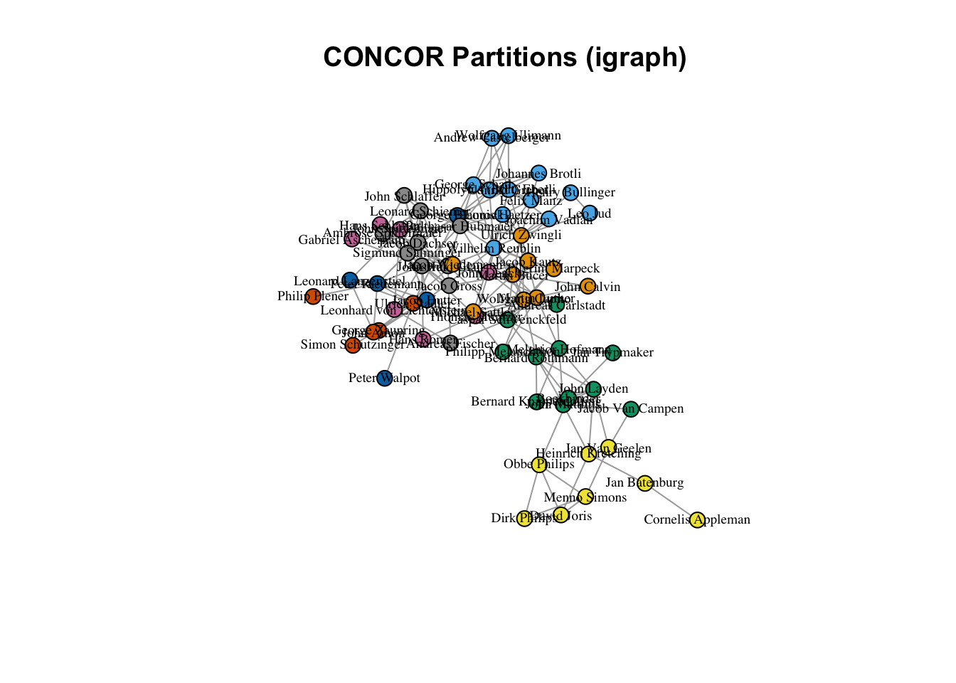
Visualize CONCOR Partitions

Code
# Extract partition information
anabaptist.par <- anabaptist.blks$block

# Plot network with CONCOLOR partitions
gplot(anabaptist.net, label=network.vertex.names(anabaptist.net), 
      label.pos=5, vertex.col=anabaptist.par, 
      label.col="black", label.cex=0.4, usearrows=FALSE,
      main="Anabaptist Network with CONCOR Partitions")

Create Blockmodel

Code
# Create blockmodel using statnet
anabaptist.bl <- blockmodel(anabaptist.net, anabaptist.blks$block)
anabaptist.bl

Network Blockmodel:

Block membership:

 1  2  3  4  5  6  7  8  9 10 11 12 13 14 15 16 17 18 19 20 21 22 23 24 25 26 
 1  1  1  2  2  2  5  2  2  2  2  2  2  2  7  7  3  8  8  1  5  1  8  8  3  7 
27 28 29 30 31 32 33 34 35 36 37 38 39 40 41 42 43 44 45 46 47 48 49 50 51 52 
 7  3  3  3  3  8  8  8  8  5  7  6  1  6  6  5  5  1  7  4  4  8  2  3  6  8 
53 54 55 56 57 58 59 60 61 62 63 64 65 66 67 
 2  4  6  4  4  7  4  3  3  3  3  1  1  4  4 

Reduced form blockmodel:

     1 2 3 4 5 6 7 8 9 10 11 12 13 14 15 16 17 18 19 20 21 22 23 24 25 26 27 28 29 30 31 32 33 34 35 36 37 38 39 40 41 42 43 44 45 46 47 48 49 50 51 52 53 54 55 56 57 58 59 60 61 62 63 64 65 66 67 
           Block 1    Block 2    Block 3    Block 4    Block 5    Block 6
Block 1 0.33333333 0.13888889 0.10101010 0.00000000 0.02222222 0.04444444
Block 2 0.13888889 0.34848485 0.00000000 0.00000000 0.06666667 0.00000000
Block 3 0.10101010 0.00000000 0.36363636 0.05681818 0.00000000 0.00000000
Block 4 0.00000000 0.00000000 0.05681818 0.35714286 0.00000000 0.00000000
Block 5 0.02222222 0.06666667 0.00000000 0.00000000 0.20000000 0.44000000
Block 6 0.04444444 0.00000000 0.00000000 0.00000000 0.44000000 0.10000000
Block 7 0.06349206 0.03571429 0.03896104 0.00000000 0.02857143 0.00000000
Block 8 0.02222222 0.03333333 0.01818182 0.00000000 0.14000000 0.00000000
           Block 7    Block 8
Block 1 0.06349206 0.02222222
Block 2 0.03571429 0.03333333
Block 3 0.03896104 0.01818182
Block 4 0.00000000 0.00000000
Block 5 0.02857143 0.14000000
Block 6 0.00000000 0.00000000
Block 7 0.14285714 0.15714286
Block 8 0.15714286 0.60000000

Density-Based Block Classification

Real-world networks rarely have perfect 1s and 0s in blocks. We use network density as a threshold to classify blocks as complete (1) or null (0).

Code
# Calculate network density
anabaptist.den <- gden(anabaptist.net, mode="graph")
anabaptist.den
[1] 0.08276798
Code
# Extract block model matrix
anabaptist.blmat <- as.matrix(anabaptist.bl$block.model)
anabaptist.blmat
           Block 1    Block 2    Block 3    Block 4    Block 5    Block 6
Block 1 0.33333333 0.13888889 0.10101010 0.00000000 0.02222222 0.04444444
Block 2 0.13888889 0.34848485 0.00000000 0.00000000 0.06666667 0.00000000
Block 3 0.10101010 0.00000000 0.36363636 0.05681818 0.00000000 0.00000000
Block 4 0.00000000 0.00000000 0.05681818 0.35714286 0.00000000 0.00000000
Block 5 0.02222222 0.06666667 0.00000000 0.00000000 0.20000000 0.44000000
Block 6 0.04444444 0.00000000 0.00000000 0.00000000 0.44000000 0.10000000
Block 7 0.06349206 0.03571429 0.03896104 0.00000000 0.02857143 0.00000000
Block 8 0.02222222 0.03333333 0.01818182 0.00000000 0.14000000 0.00000000
           Block 7    Block 8
Block 1 0.06349206 0.02222222
Block 2 0.03571429 0.03333333
Block 3 0.03896104 0.01818182
Block 4 0.00000000 0.00000000
Block 5 0.02857143 0.14000000
Block 6 0.00000000 0.00000000
Block 7 0.14285714 0.15714286
Block 8 0.15714286 0.60000000
Code
# Apply density threshold
anabaptist.blmat[anabaptist.blmat < anabaptist.den] <- 0
anabaptist.blmat[anabaptist.blmat >= anabaptist.den] <- 1
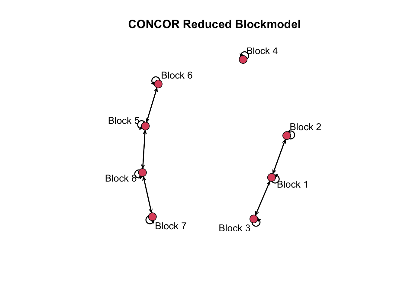
anabaptist.blmat
        Block 1 Block 2 Block 3 Block 4 Block 5 Block 6 Block 7 Block 8
Block 1       1       1       1       0       0       0       0       0
Block 2       1       1       0       0       0       0       0       0
Block 3       1       0       1       0       0       0       0       0
Block 4       0       0       0       1       0       0       0       0
Block 5       0       0       0       0       1       1       0       1
Block 6       0       0       0       0       1       1       0       0
Block 7       0       0       0       0       0       0       1       1
Block 8       0       0       0       0       1       0       1       1

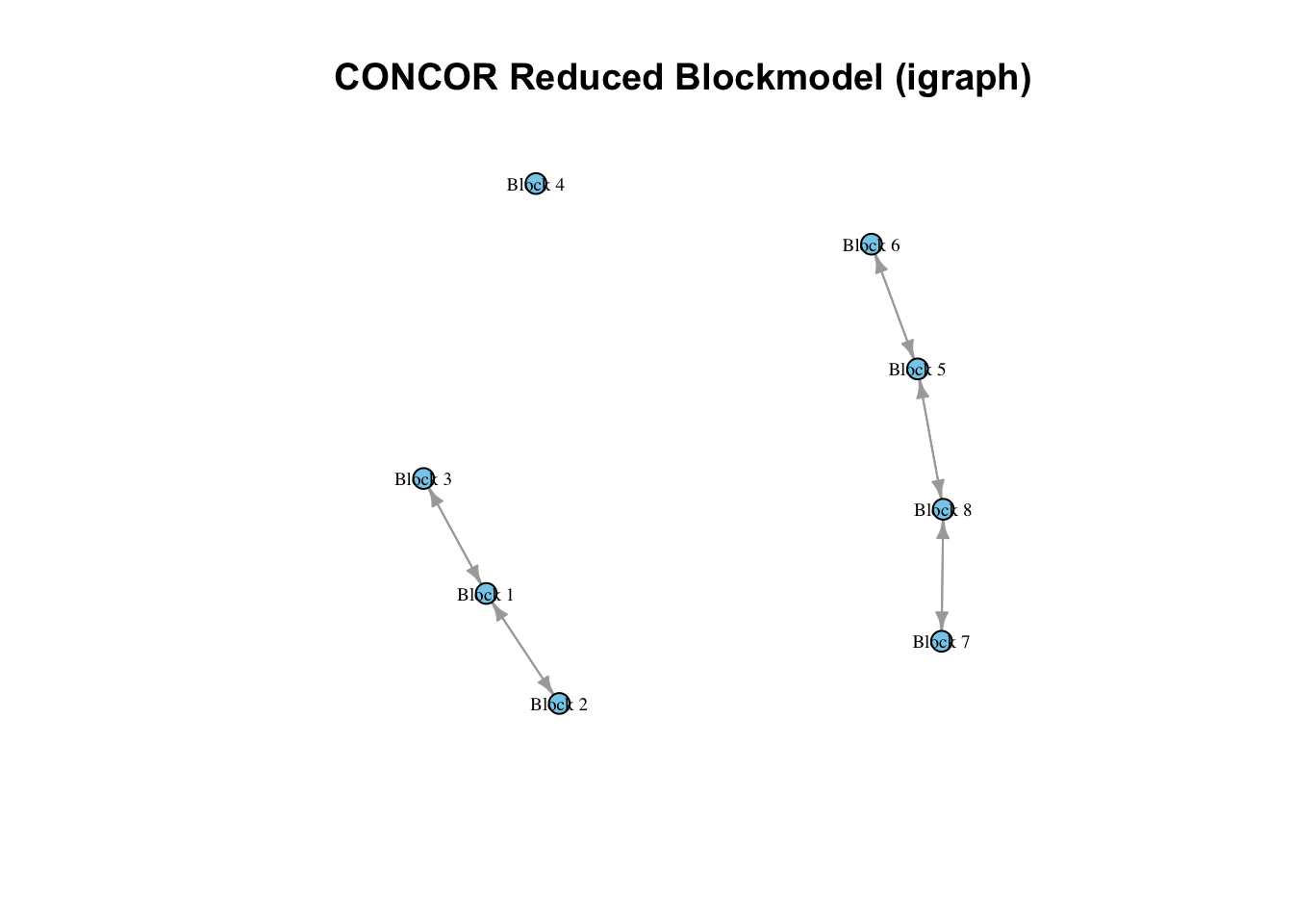
Visualize Reduced Blockmodel

Code
# Create and plot reduced network
anabaptist.blnet <- as.network(anabaptist.blmat)
gplot(anabaptist.blmat, usearrows=TRUE, arrowhead.cex=0.5,
      label=network.vertex.names(anabaptist.blnet), 
      diag=TRUE, loop.cex=1,
      main="CONCOR Reduced Blockmodel")

Method 3: Optimization Approach

The optimization approach uses random partitions and iteratively improves the fit by minimizing error scores.

Run Optimization Algorithm

Code
#dim(anabaptist.mat)
# Run optimization with 8 blocks
anabaptist.opt <- optRandomParC(M=anabaptist.mat, k=8, rep=500, 
                                approaches="bin", blocks=c("nul","com"))


Starting optimization of the partiton 50 of 500 partitions.


Starting optimization of the partiton 100 of 500 partitions.


Starting optimization of the partiton 150 of 500 partitions.


Starting optimization of the partiton 200 of 500 partitions.


Starting optimization of the partiton 250 of 500 partitions.


Starting optimization of the partiton 300 of 500 partitions.


Starting optimization of the partiton 350 of 500 partitions.


Starting optimization of the partiton 400 of 500 partitions.


Starting optimization of the partiton 450 of 500 partitions.


Starting optimization of the partiton 500 of 500 partitions.


Optimization of all partitions completed
2 solution(s) with minimal error = 254 found. 
Code
# Display optimization results
anabaptist.opt
Network size: 67 

Approachs (paramter): bin
Blocks (paramter)
nul com 

Sizes of clusters:
 1  2  3  4  5  6  7  8 
 1  7  1 37  4  6  3  8 

IM
    1   2   3   4   5   6   7   8
1 nul com com nul com nul nul nul
2 com com nul nul nul nul nul nul
3 com nul nul nul com nul com com
4 nul nul nul nul nul nul nul nul
5 com nul com nul nul nul com nul
6 nul nul nul nul nul com nul nul
7 nul nul com nul com nul com nul
8 nul nul com nul nul nul nul nul

Error: 254 
2 solutions with minimal error exits. Only results for the first one are shown above!

Visualize Permuted Matrix

Code
# Plot permuted matrix
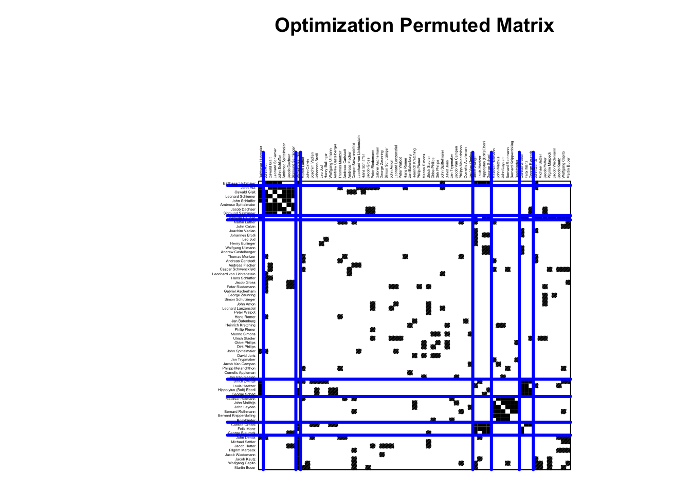
plot(anabaptist.opt, main="Optimization Permuted Matrix")

Extract and Apply Partitions

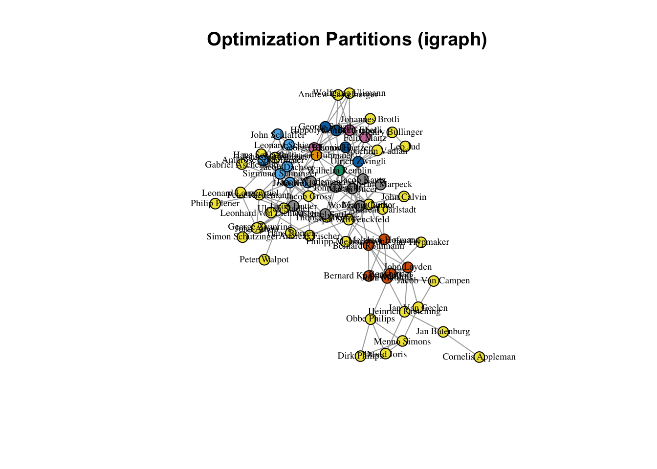
Code
# Extract best partition
anabaptist.best1 <- anabaptist.opt$best$best1$clu

# Plot network with optimization partitions
coord <- gplot(anabaptist.net, label=network.vertex.names(anabaptist.net),
               label.pos=5, vertex.col=anabaptist.best1, 
               label.col="black", label.cex=0.4, usearrows=FALSE,
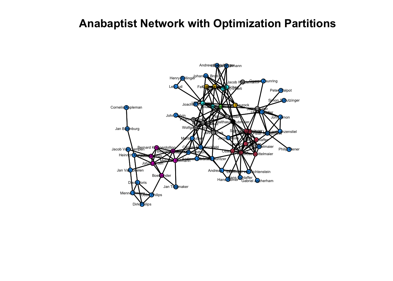
               main="Anabaptist Network with Optimization Partitions")

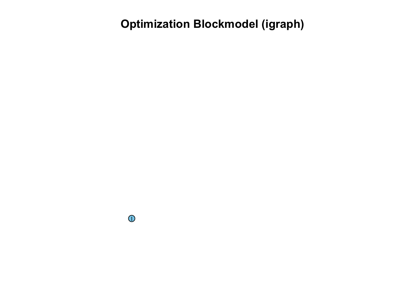
Create Image Matrix

Code
# Create image matrix from optimization results
anabaptist.optim <- IM(anabaptist.opt)
anabaptist.optim <- as.matrix(anabaptist.optim[[1]])
anabaptist.optim
     [,1] 
[1,] "nul"
Code
# Convert to binary matrix
anabaptist.optim[anabaptist.optim == "nul"] <- 0
anabaptist.optim[anabaptist.optim == "com"] <- 1

# Create and plot optimization network
anabaptist.optnet <- as.network(anabaptist.optim, loops=TRUE)
gplot(anabaptist.optnet, arrowhead.cex=0.5, 
      label=network.vertex.names(anabaptist.optnet),
      diag=TRUE, loop.cex=1, label.pos=5,
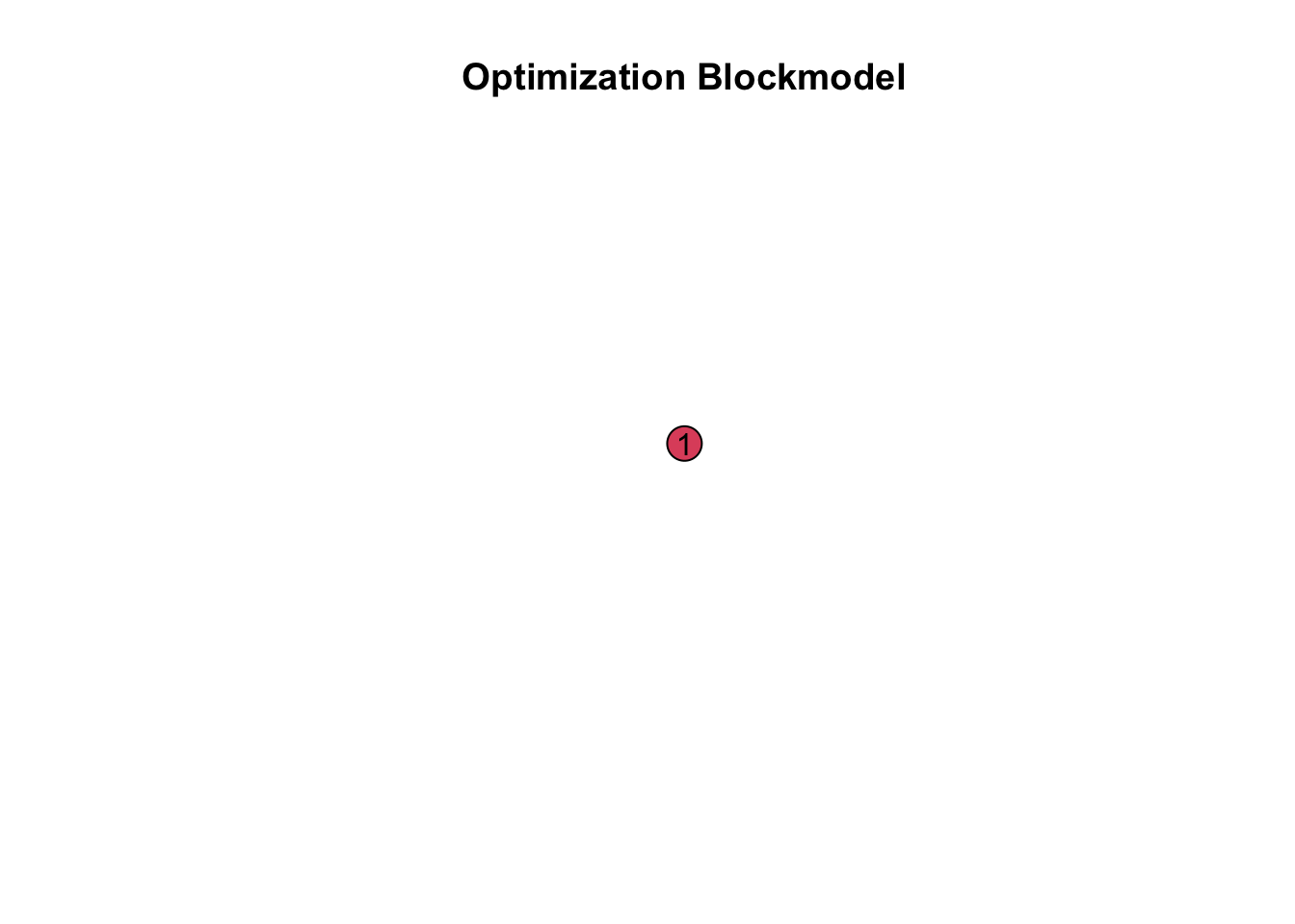
      main="Optimization Blockmodel")

Compare Different Partition Sizes

Code
# Run optimization with 12 blocks
anabaptist.opt2 <- optRandomParC(M=anabaptist.mat, k=12, rep=500,
                                 approaches="bin", blocks=c("nul","com"))


Starting optimization of the partiton 50 of 500 partitions.


Starting optimization of the partiton 100 of 500 partitions.


Starting optimization of the partiton 150 of 500 partitions.


Starting optimization of the partiton 200 of 500 partitions.


Starting optimization of the partiton 250 of 500 partitions.


Starting optimization of the partiton 300 of 500 partitions.


Starting optimization of the partiton 350 of 500 partitions.


Starting optimization of the partiton 400 of 500 partitions.


Starting optimization of the partiton 450 of 500 partitions.


Starting optimization of the partiton 500 of 500 partitions.


Optimization of all partitions completed
1 solution(s) with minimal error = 222 found. 
Code
# Compare error scores
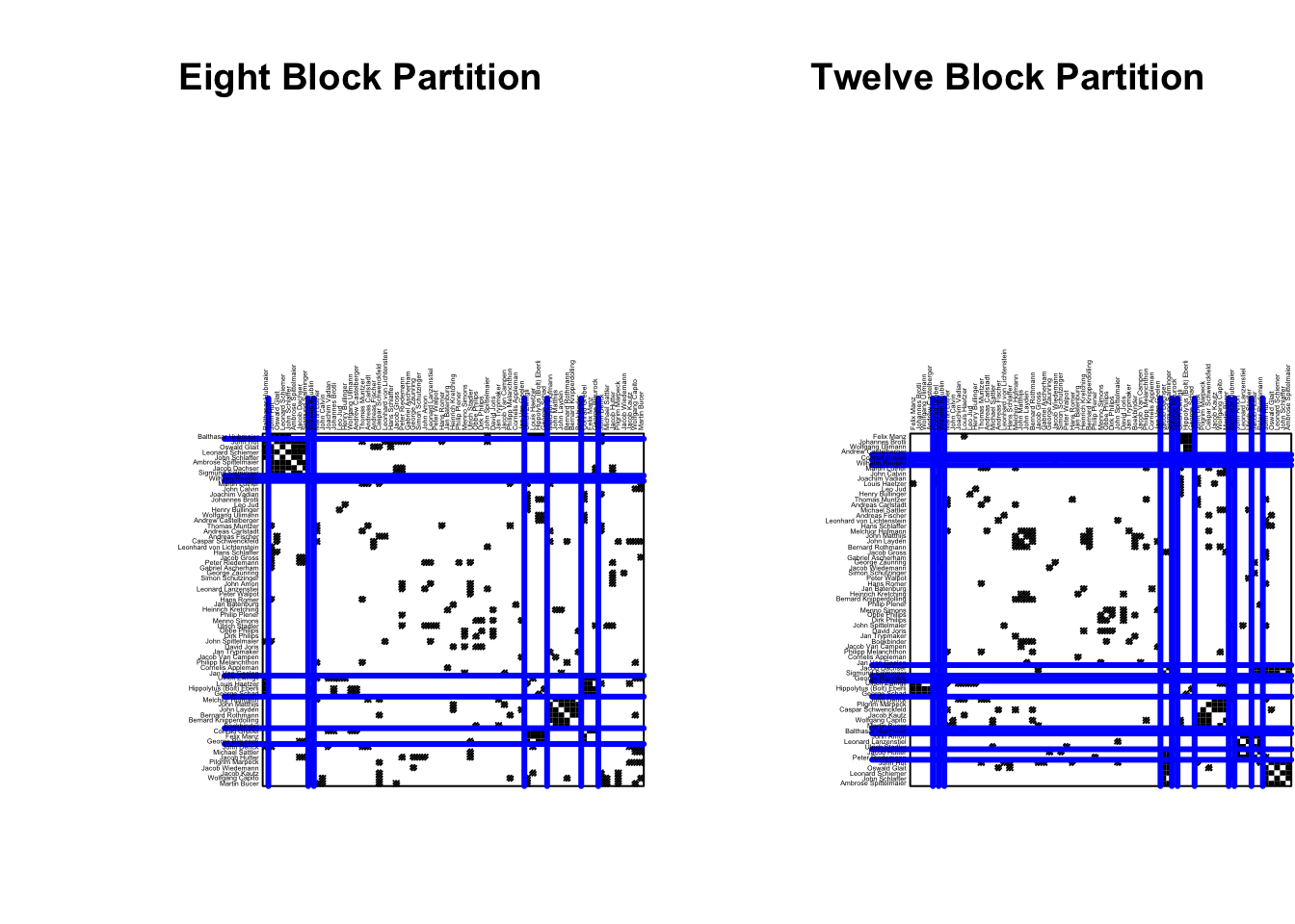
cat("8-block error:", anabaptist.opt$best$best1$err, "\n")
8-block error: 254 
Code
cat("12-block error:", anabaptist.opt2$best$best1$err, "\n")
12-block error: 222 
Code
# Plot comparison
par(mfrow=c(1,2))
plot(anabaptist.opt, main="")
title("Eight Block Partition")
plot(anabaptist.opt2, main="")
title("Twelve Block Partition")

Code
par(mfrow=c(1,1))

igraph Visualizations

Code
# Detach sna and load igraph
detach("package:sna", unload=TRUE)
library(igraph)
library(intergraph)

# Convert to igraph objects
anabaptist.ig <- asIgraph(anabaptist.net)
anabaptist.blig <- asIgraph(anabaptist.blnet)
anabaptist.optig <- asIgraph(anabaptist.optnet)

# Assign labels
V(anabaptist.ig)$label <- V(anabaptist.ig)$vertex.names
V(anabaptist.blig)$label <- V(anabaptist.blig)$vertex.names
V(anabaptist.optig)$label <- V(anabaptist.optig)$vertex.names

# Set layout
anabaptist.ig$layout <- layout.kamada.kawai(anabaptist.ig)

CONCOR Partition in igraph

Code
plot(anabaptist.ig, vertex.label.cex=0.6, vertex.label.color="black",
     edge.arrow.mode=0, vertex.color=anabaptist.par, vertex.size=8,
     main="CONCOR Partitions (igraph)")

Optimization Partition in igraph

Code
plot(anabaptist.ig, vertex.label.cex=0.6, vertex.label.color="black",
     edge.arrow.mode=0, vertex.color=anabaptist.best1, vertex.size=8,
     main="Optimization Partitions (igraph)")

Reduced Blockmodels in igraph

Code
# CONCOR blockmodel
coords1 <- layout.kamada.kawai(anabaptist.blig)
plot(anabaptist.blig, vertex.label.cex=0.6, vertex.label.color="black",
     edge.arrow.size=0.5, vertex.color="Sky Blue", vertex.size=8,
     main="CONCOR Reduced Blockmodel (igraph)")

Code
# Optimization blockmodel  
coords2 <- layout.kamada.kawai(anabaptist.optig)
plot(anabaptist.optig, vertex.label.cex=0.6, vertex.label.color="black",
     edge.arrow.size=0.5, vertex.color="Sky Blue", vertex.size=8,
     main="Optimization Blockmodel (igraph)")

Theoretical Framework: Structural Equivalence

Key Concepts

Structural Equivalence occurs when two actors have identical patterns of relationships with all other actors in the network. Actors who are structurally equivalent are perfect substitutes for one another in terms of their network positions.

Methodological Approaches

  1. Euclidean Distance: Measures direct dissimilarity between connection patterns

  2. CONCOR: Uses iterative correlations to identify structurally similar positions

  3. Optimization: Iteratively improves partition fit by minimizing error scores

Blockmodeling Interpretation

  • Complete Blocks (1-blocks): Dense connection patterns within position

  • Null Blocks (0-blocks): Sparse or absent connections between positions

  • Image Matrix: Simplified representation of connection patterns between positions

Practical Applications

Structural equivalence analysis helps identify:

  • Functional roles within organizations

  • Competitive positions in markets

  • Redundancy in communication networks

  • Potential for substitution or replacement

Conclusion

This lab demonstrated three complementary approaches to structural equivalence analysis:

  1. Euclidean Distance provides a straightforward dissimilarity measure

  2. CONCOR offers a robust correlation-based partitioning method

  3. Optimization delivers empirically-driven best-fit solutions

Each method has strengths and is appropriate for different analytical contexts. The choice among them depends on research questions, network characteristics, and theoretical frameworks.

References

  • Wasserman, S., & Faust, K. (1994). Social Network Analysis: Methods and Applications. Cambridge University Press.

  • Breiger, R. L., Boorman, S. A., & Arabie, P. (1975). An algorithm for clustering relational data with applications to social network analysis. Journal of Mathematical Psychology, 12, 328-383.

  • Ziberna, A. (2007). Generalized blockmodeling of valued networks. Social Networks, 29, 105-126.

  • Burt, R. S. (1976). Positions in networks. Social Forces, 55, 93-122.