Summary
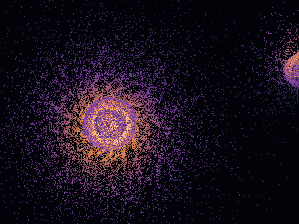
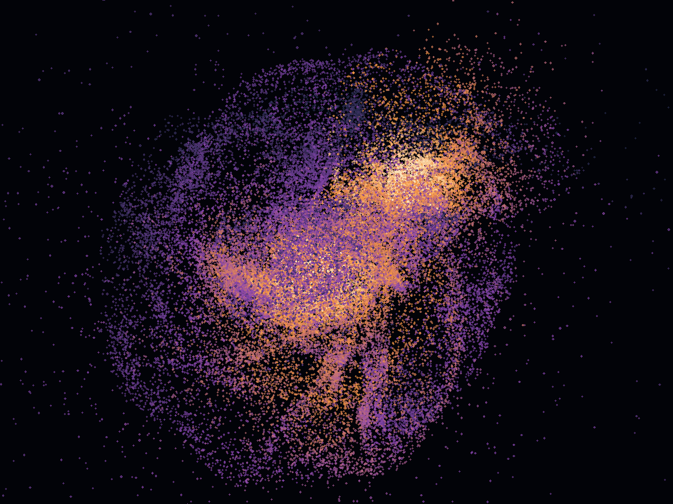
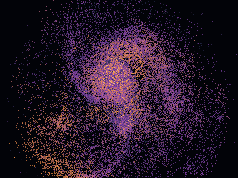
We implemented a 3D Barnes-Hut based N-Body Galaxy Simulator in CUDA on the GPU, targeting large simulations of as many as a million bodies in various configurations, including simulating regular Plummer-disk galaxy behaviors and spiral-galaxy formations. We developed, benchmarked and analyzed two CPU implementations and four GPU implementations with progressively better performance: (v-1) running the entire galaxy simulation in O(N^2) time, used for validation; (v0) which is the serial Barnes-Hut implementation on the CPU; (v1) where the largest bottle neck on CPU, the tree-walk and force calculations, are moved to the GPU; (v2) where we attempted moving the next biggest bottleneck, the octree construction, to GPU using Burtscher [2]; (v3) which redoes the octree construction using a different level-by-level approach; and finally (v4) where we optimize force calculation by minimizing warp divergence. CPU benchmarking was performed on a 13th Gen Intel(R) Core(TM) i5-13600K, while the GPU used is an NVIDIA RTX 3070. We plan on showcasing our optimizations, some of the intuitions behind them visually, and a few simulations of disc-shaped galaxies colliding to form spiral-shaped ones.
Background
Problem
The N-body galaxy simulation problem evolves a system of N point masses under the effects of gravity. While exact calculations require computing the effects of interactions between every pair of bodies with computational complexity O(N^2), Barnes-Hut [1] approximates far away body clusters as a single point mass at their center of mass (CoM) to reduce the complexity. They define a cell as a region of space containing point masses, and divide all of space into cells using octrees. They start with a single cell covering all of the simulated space, and keep dividing the cell into smaller and smaller octants until every smallest cell has at most 1 point mass in it. They also define a parameter theta which decides at what relative size of cell to the distance from a mass do we approximate the entire cell as a single point. theta is in fact an approximation of the angle subtended by the cell at the mass we’re calculating forces for.
if cell_width / distance < theta
then use cluster's COM as point mass
else recurse into cluster's 8 sub-cells
Key Data Structures
We need two main structures, one to represent the bodies that are provided as input, and the other to represent the octree that we construct and walk along for force calculations:
- Bodies array: we use a structure-of-arrays layout here, where position
(x,y,z), velocity(vx, vy, vz), and mass(m)are stored in separate arrays within the same struct. This is done to allow for memory coalescing as consecutive warp threads access consecutive elements in each of these arrays simultaneously.
- The octree: this is the 8-ary tree we use to partition all of (simulated) space into cells, such that each cell has at most 1 point mass in it. Each internal node represents a cube of space and has up to 8 children, one per octant. Each node stores its cube’s center, half-width, CoM, total mass, body count, depth, and the eight child pointers. All of these are of course stored in the struct-of-arrays format. The children pointers are actually implemented as indices into the appropriate array.
Key Operations per Timestep
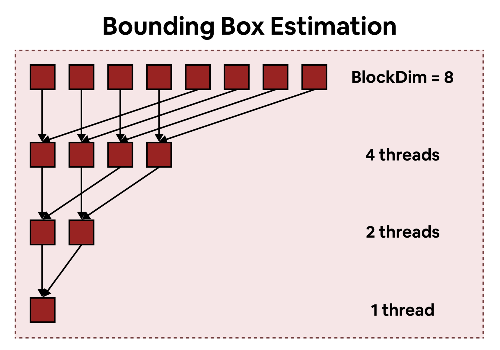
- Drawing bounding boxes (BBs): compute BBs of all bodies in a reduction operation that looks very much like the one we used in Assignment 2 for prefix sum
- Build tree root: reduce per-body BBs into a single large BB to obtain the extent of the entire space under simulation and create the octree’s root
- Tree building: build the octree layer by layer from top to bottom, partitioning the bodies into their appropriate cells
- CoM calculations: traverse the tree layer by layer from bottom to top, computing CoM for every node/body in the layer
- Force traversal: for each body, walk the entire tree, deciding at each visited node whether to descend further or not based on theta
- Integration: apply the forces to move the bodies, which we do with a simple integrator like Kick Drift, using equations v += at and x += vt, where x is position, v is velocity, and a is acceleration.
Inputs and Outputs
The inputs are the N bodies, along with time step size dt, approximation parameter theta, gravitational constant G, and the number of steps for the simulation n_steps. We also pass a parameter softening used to handle precision issues when calculating inverse distances (since Newtonian gravity approaches a singularity as the distance between two bodies approaches zero, leading to numerical instability in the simulation.
The program outputs the positions of the N bodies after the n_steps time steps, with an option to output them after every k steps for the purpose of validation or visualization.
Profiling Results and Parallelizability
We first tested our serial CPU implementation of Barnes-Hut and observed that almost all the time (> 97\%) is spent on the force calculations:
Given this observation, we first focused on parallelizing the tree walk and force calculations on the GPU, hoping to use 1 GPU thread per body and parallelize the entire process. As force calculations at each body are independent of other bodies in a given time step, we can potentially leverage all threads in the GPU to run all N bodies simultaneously. This is thus, at least in theory, highly amenable to SIMT execution. Another great benefit of such a division of work is that each thread can independently perform integration on its own body once it has computed the force without having to wait for the other other threads to complete their force computations. However, as we later see, the workload is quite irregular and requires some optimizations to achieve good performance.
Once we optimized the force calculation step, the tree construction became the bottleneck (thanks to Amdahl’s Law of course). Here, the tree structure itself is the dependency constraint: bodies inserted into disjoint subtrees don’t contend on any shared resource except the tree’s root, while bodies in subtrees with significant overlap face larger contention. The workload is thus highly irregular, and required careful consideration to optimize to make it amenable to SIMT.
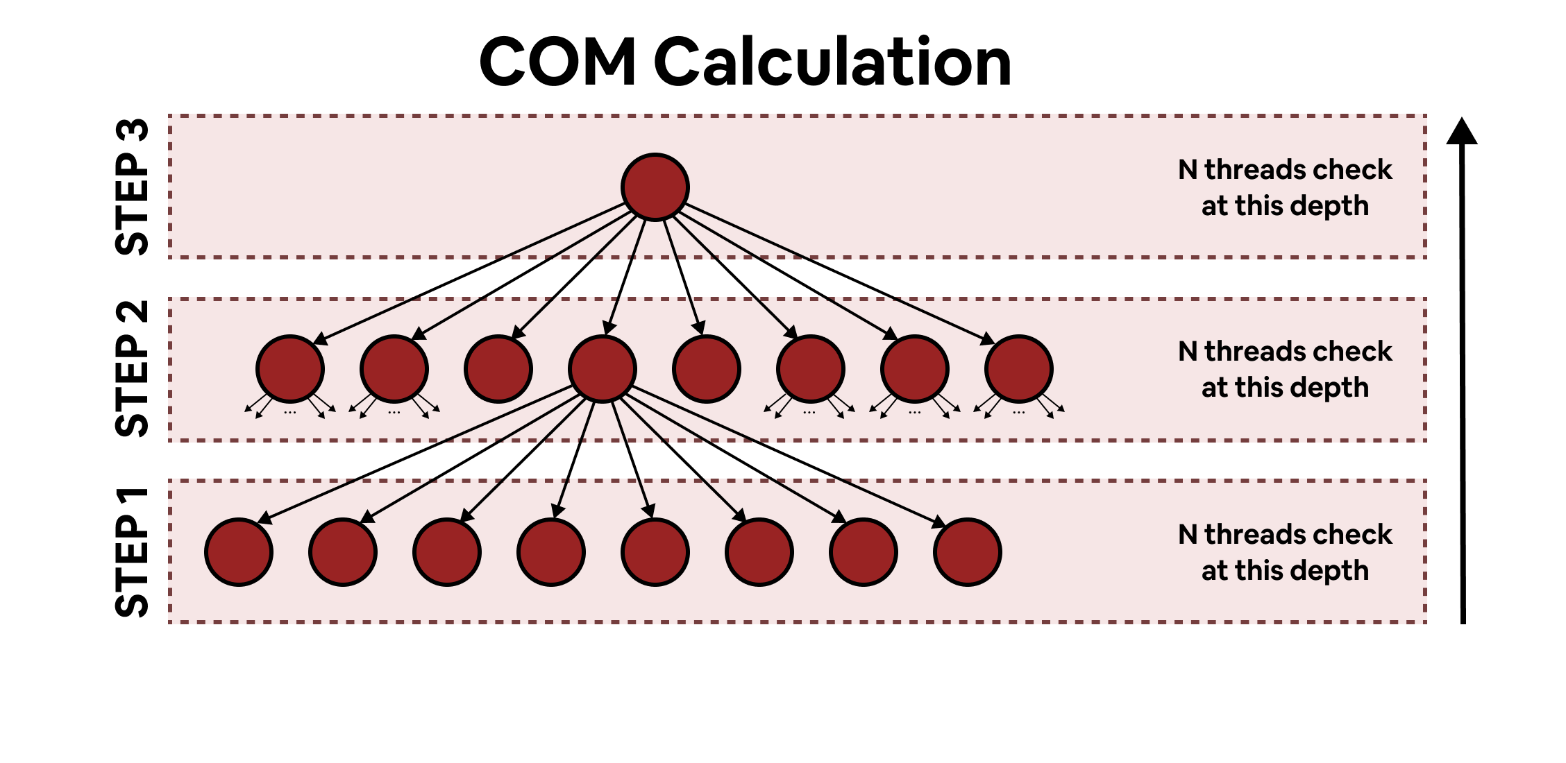
Moving the tree construction to the GPU, also requires moving the intermediate CoM calculation step to the GPU as well. This operation is again inherently tied to the tree structure, but when viewed as a layer-by-layer operation (i.e. operating on nodes of only a certain depth at any given time), it is parallelisable as bodies at the same depth don’t depend on each other for their CoM. It is, however, a serial computation across depths. Thus we process the CoM calculation depth-wise for maximum compatibility with SIMT execution.
There is also scope for significant spatial locality throughout the algorithm. Bodies that are spatially close tend to traverse the same portions of the tree. So if threads in a warp process such spatially close bodies, they can coalesce many of their loads and also minimise warp divergence by having near-identical traversal paths. In order to exploit this, we sort the bodies by their Morton-Code which linearizes 3D positions so that consecutive indices in the bodies array correspond to consecutive cells along a space-filling curve. This is an idea that we used in Assignment 4 to improve spatial locality of wires, and is also used by Karras [3].
Approach
Target platform and tools
- Language/APIs: C++17, CUDA 12.4, Thrust (radix sort), Nsight Systems for profiling
- Hardware: GPU: RTX 3070 (46 SMs, 5888 CUDA cores, 8 GB GDDR6); CPU: 13th Gen Intel(R) Core(TM) i5-13600K
- Build:
makewith sm_86,-O3
Implementations
v1: CPU tree + GPU force
Breakdown of each step:
- Build entire octree on CPU using the bodies array
- Tree and bodies copied to GPU
- GPU launches one thread per body, where each thread walks the tree using a private stack of 256 integers. It uses the standard theta criterion while accumulating forces into the registers
- Updated bodies copied back to CPU
- GOTO step 1
In order to make the most use of the GPU, we map one thread per body, 256 threads per block, with ceil(N/256) blocks. Each thread’s stack is in per-thread global memory as it was too large to fit into the registers. However, load coalescing is poor, as each of the 32 threads in the warp process arbitrary bodies that may not be spatially close.
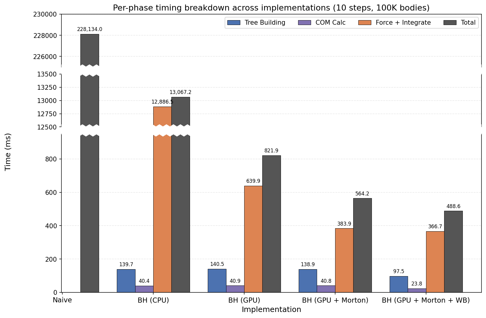
This gave us our first observation/idea: sort the bodies to exploit cache locality. We reordered the bodies based on a Morton-Code embedding of their positions. Morton-Code takes a 3-D floating point vector and converts it into a 63-bit integer, where bits 3i, 3i+1, 3i+2 correspond to the octant at depth i . Thus, sorting bodies by their Morton-Code provides a natural spatial ordering, leading to improved cache locality. We saw force calculation times drop from 640 ms to 384 ms on 100K bodies (RTX 2080) on using Morton-Codes, as mentioned in the mid-term report. We also kept the morton-ordered bodies across steps, which led to CPU tree build times also going down from 140ms to 98ms (GHC machine). Cache locality was a huge win!!
However, we also observed that now the tree construction became the bottleneck. On simulating 1M bodies in a Plummer disc, we observed tree construction taking ~185ms of 800ms total time, or 23%. We thus moved to optimizing the tree construction next.
v2: Tree construction on the GPU using Burtscher [2]
We moved tree construction to the GPU following the outline in Burtscher [2]:
- One thread per body: each thread descends from the root, at each level performing
atomicCAS(&children[octant][parent], EMPTY, LOCKED)to claim a slot, writing the body ref, then unlocking.
- On collision (slot already holds a body): the locking thread allocates child nodes via
atomicAdd(node_count, 1), sub-divides until the two bodies separate, and unlinks the lock. ⇒ Lock held until bodies separated
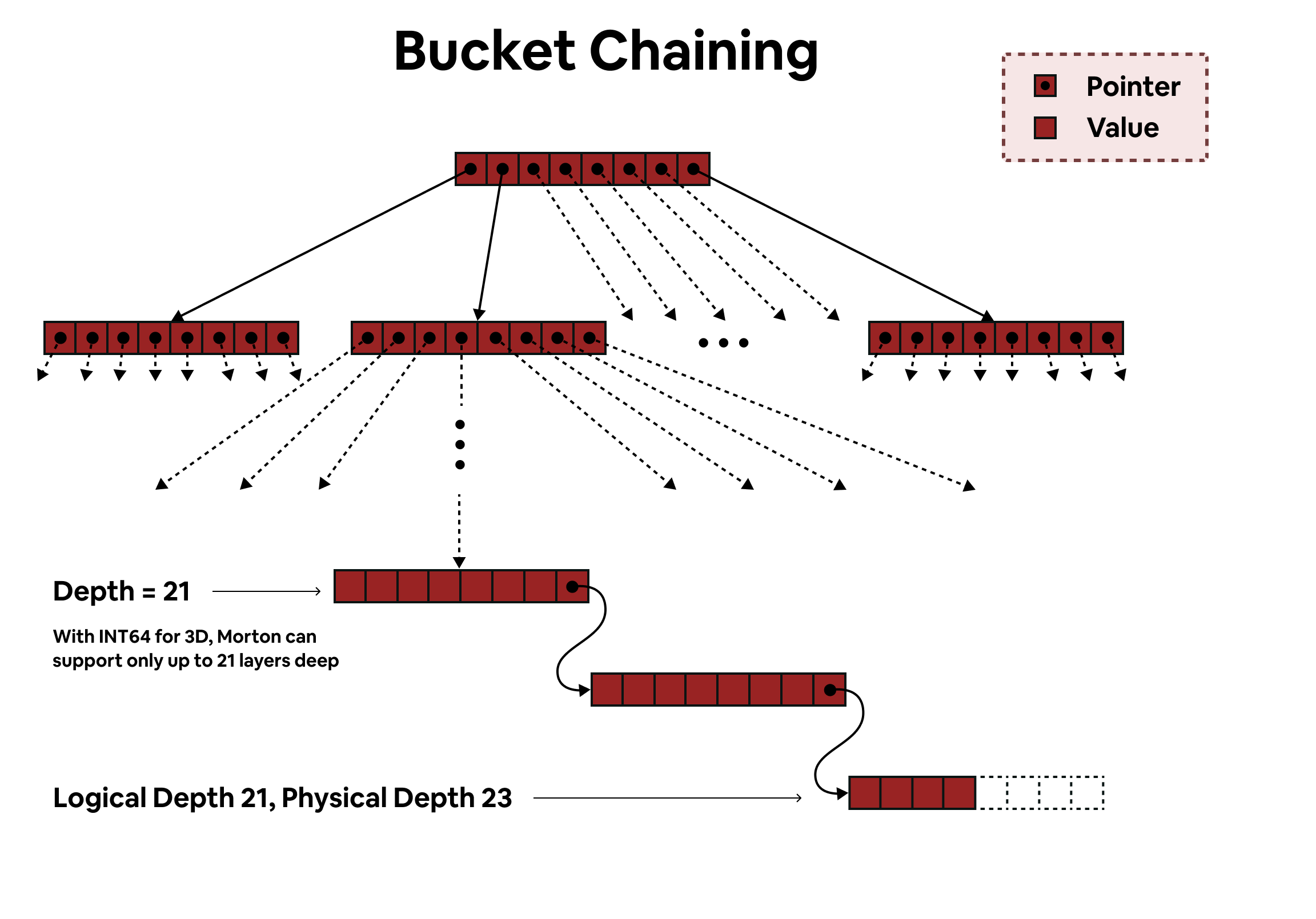
- Bucket chains at depth 32 to handle near-coincident bodies
While we expected this to be fast as suggested in the paper, we were taken aback to find the 1M Plummer simulation now spent ~6500ms on tree construction, roughly 65x slower than the CPU-based construction (100ms on i5-13600k). Even on 8k bodies it took ~9s when we expect the entire simulation to complete in about 200ms. Thus it was obvious we were doing something seriously wrong, and analysis lead to the obvious culprit: our locks have huge contention.
This is funnily similar to the problem on the first exam, where a million threads all contended on a handful of locks. In our implementation, 1M threads (for N = 1M) all tried to lock one of the 8 children of the root node to insert themselves. And then they try to lock the up to 64 children at depth 2, and 512 children at depth 3 and so on. The contention and blocking of waiting threads led to extreme slowdowns. We had to get rid of the locking.
v3: Tree construction, one level at a time
In order to get rid of the contention created by locks, we drew inspiration from Lauterbach et al. [4] to instead construct the tree one level at a time. The pipeline now looks like:
- Bounding box and root init: as described earlier, using one reduction kernel to calculate individual body BBs, and one reduction kernel to obtain the overall space’s bounding box
- Compute morton codes of each position: using standard morton code algorithm, mapping each position to an integer corresponding to a point in the [0, 2^{21})^3 integer grid.
- Sort bodies by morton code position: using
thrust::sort_by_key, which solves the problem using CUB radix sort. (this part has no contention and is BW bound). Then reorder the bodies using the sorted keys.
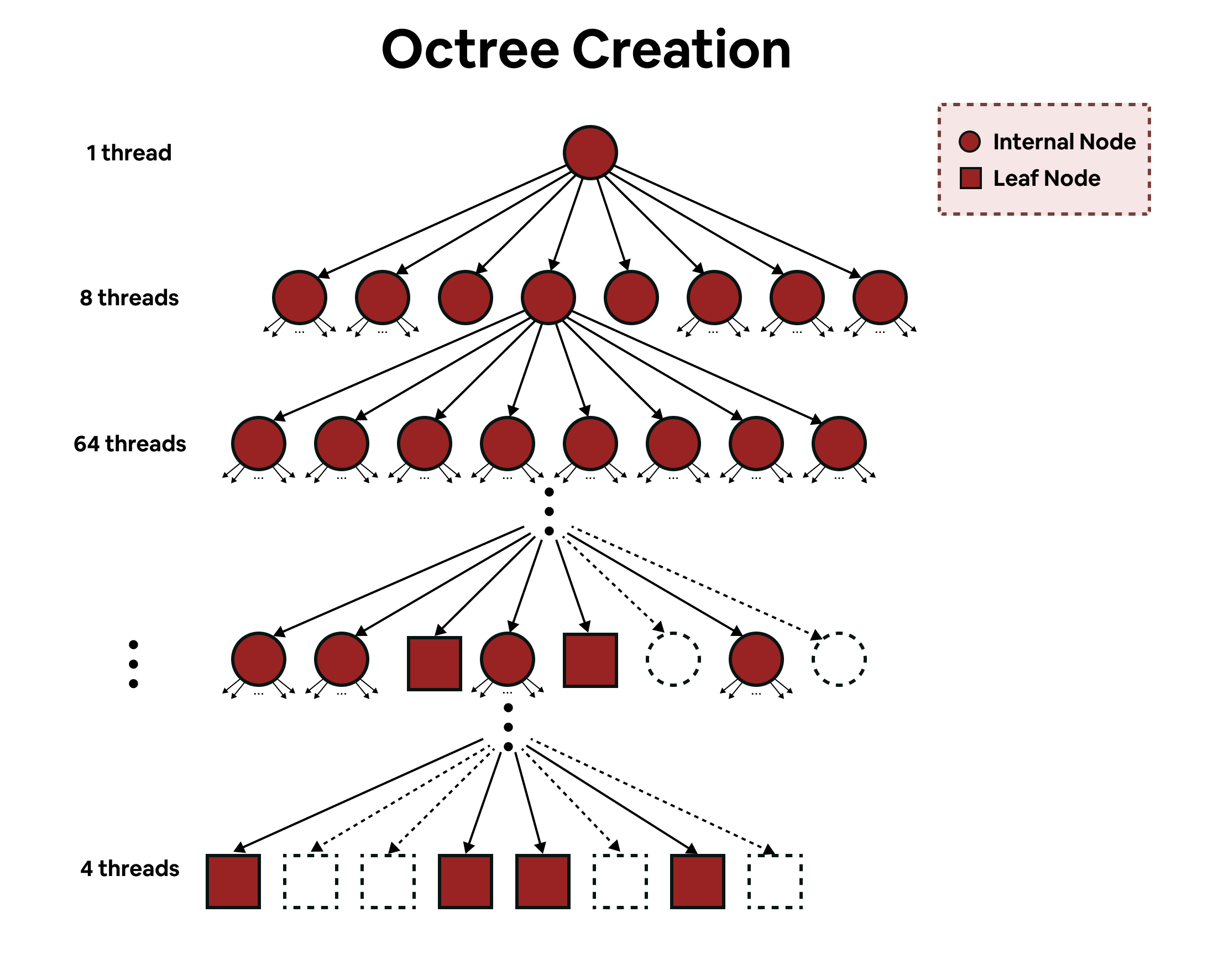
- Build tree level by level: run one thread for every cell that is active at the current depth being constructed. Each cell is a triple of
(lo, hi, node_idx)which means its parent isnode_idxand it contains bodies[lo, hi). Every thread does binary search on the Morton sorted array to find its children’s 8 octant boundaries, then for each non-empty sub-range, it moves the corresponding bodies into that octant’s cell. Cells with more than 1 body have to be further divided and are thus pushed into the next level’s work queue. Keep doing this for a max depth of 21, beyond which bodies in the same cell all have the same Morton code and must thus be chained together, much like a hash table. In order to implement the work queue, we use double-buffered arrays, each switching between roles of input and output to the build tree kernel.
- CoM: perform as described earlier, going up from the deepest level. Every body is assigned a thread, and only threads of bodies present at the current depth compute the CoM, as it is guaranteed all lower cells’ CoMs have been processed. Once done, go up a depth and repeat until you reach the root. At the root, exactly one thread will be active,
tid = 0.
- Force-calculations: using the same approach as in v1
And here we immediately saw huge improvements in the tree construction times. For example, with 1M bodies, construction times went down from ~1750ms in v1 to ~19ms in v3. A huge win!
Tree construction times for Plummer Discs, theta = 0.1
| Bodies | v1 Tree (ms) | v3 Tree (ms) | Speedup |
|---|---|---|---|
| 1K | 0.6 | 2.1 | 0.29x |
| 10K | 7.6 | 3.2 | 2.38x |
| 100K | 91.5 | 6.4 | 14.30x |
| 1M | 1749.3 | 19.1 | 91.59x |
We observe that v3 performs slightly worse in very small test cases, and can be attributed to overheads to constructing the tree on the GPU, including launching kernels, extra cudaMalloc, and data transfer.
By keeping #threads launched at every depth limited to the #cells at that level, we have effectively mapped well to the hardware constraints of having poor lock implementations. We have instead replaced the locks with atomicAdd which atomically fetches for each thread the next child’s position in a pre-allocated array.
Also, each thread now works on subdividing a unique cell that it has received in the current work queue with index in[tid], so all modifications it makes are to add children to this node by accessing children[oct][in[tid]] . Thus, threads make disjoint accesses to the shared data structure, and no locks are required.
v4: Reducing warp-divergence in the force calculation kernel
Run times for Plummer Discs, theta = 0.1
| Version | Tree (ms) | CoM (ms) | Force (ms) | Total (ms) |
|---|---|---|---|---|
| v1 | 91.5 | 20.4 | 14941.0 | 15052.8 |
| v3 | 6.4 | 1.1 | 22651.8 | 22798.5 |
Notice that the while the tree construction and CoM times has become negligible on the GPU, our force calculation times have gone up. While initially strange, Nsight measurements helped.
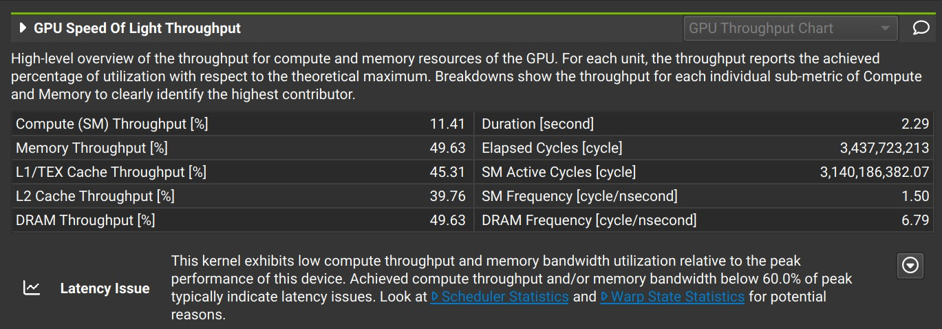
Analysing the performance of v3 on N=100k, theta = 0.1 showed us that the force kernel was heavily DRAM-bound, with compute TP at a meagre 11%. While the occupancy is quite high at 80%, we also tried to improve on that while optimizing the performance.
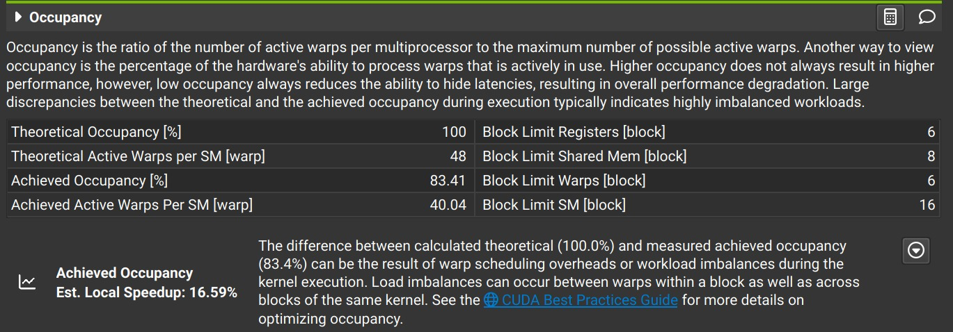
Looking at the code, we came up with some potential pain points:
- Local memory stack creating too many and too frequent global memory transactions, making it memory bound
- Threads within a warp all making the same loads when traversing the tree, leading to redundant traffic
To solve these, we use the fact that bodies spatially close to each other have to perform the same tree walk:
- Use a per-warp stack in shared memory, written to only by lane 0: this way, only 1 lane does all the stack push/pop operations, reducing the memory BW requirements by 32x. Further, now moving the stack from global per-thread memory to shared memory, we have inherently increased performance.
In order to perform the same tree walk across the entire warp, however, we need to slightly alter the original Barnes-Hut: usually, every body independently decides whether it should continue exploring the tree down, or stop at a particular node based on theta. To prevent this and ensure every lane in the warp walks the same path, we reduce the approximation by always exploring down the tree unless every lane in the warp agrees to approximate a particular node. So if only some lanes want to approximate, they are not allowed to and continue going down the tree. Thus, we have increased the accuracy of the simulation and increased the workload, but by doing so, we see huge gains in the force calculation performance.
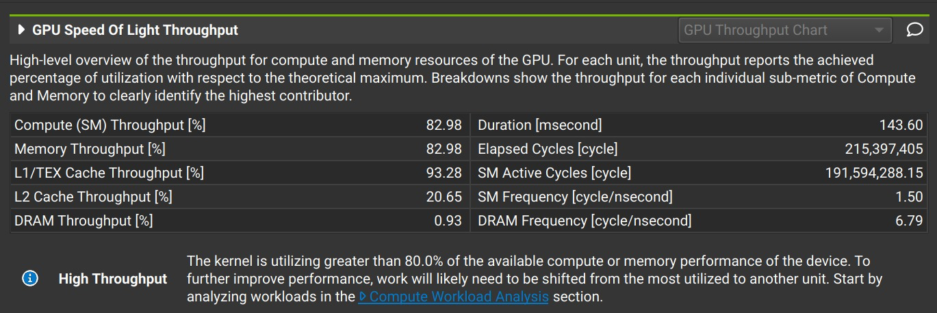
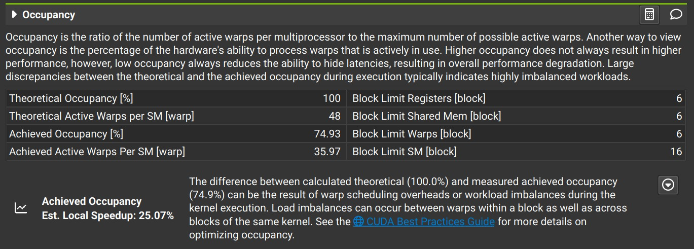
The Nsight results show now the compute TP has gone up to 83%, and DRAM TP to < 1%. This clearly explains why v3 performed so poorly, and how our optimization helped improve the performance by eliminating global transactions that go to DRAM. By using a stack in the shared memory, we have greatly reduced latencies and improved performance.
Note however that we have made a small tradeoff. By these changes, we have reduced the occupancy slightly to ~75%. This comes partly from lane 0 doing a lot of work that other lanes do not. However the tradeoff is asymmetric in terms of performance gains. We leave the exploration of improving occupancy while maintaining performance for future work.
Results
Experimental Setup
- Hardware: GPU: RTX 3070 (8 GB, sm_86, 46 SMs); CPU: 13th Gen Intel(R) Core(TM) i5-13600K
- Inputs: Plummer-disk distributions at N = 10K, 100K, 1M. Generated using inverse-CDF sampling
- Parameters:
dt = 0.001, theta = 0.1, softening = 0.01, G = 1.0.
- Measurement: wall-clock time via
cudaEvents for per-kernel breakdown
- Baseline: CPU Barnes-Hut (single-threaded)
- Correctness:
./validateruns the same input through naive O(N^2) and Barnes–Hut, and reports maximum relative position/velocity error vs. naive
Plummer Disk, with 1k bodies, theta=0.1
| Method | Tree (ms) | COM (ms) | Force + Int (ms) | Total (ms) | Speedup vs Serial |
|---|---|---|---|---|---|
| Serial | 0.7 | 0.2 | 45.1 | 46.0 | 1.00x |
| v1: CPU Tree + GPU Force | 0.6 | 0.1 | 234.7 | 235.4 | 0.20x |
| v3: GPU Tree + Force | 2.1 | 0.5 | 27.6 | 170.2 | 0.27x |
| v4: GPU Tree + Force warp opt | 2.0 | 0.5 | 5.1 | 149.3 | 0.31x |
Plummer Disk, with 10k bodies, theta=0.1
| Method | Tree (ms) | COM (ms) | Force + Int (ms) | Total (ms) | Speedup vs Serial |
|---|---|---|---|---|---|
| Serial | 7.3 | 1.7 | 8998.6 | 9007.6 | 1.00x |
| v1: CPU Tree + GPU Force | 7.6 | 1.7 | 261.4 | 270.7 | 33.27x |
| v3: GPU Tree + Force | 3.2 | 0.7 | 785.5 | 936.7 | 9.62x |
| v4: GPU Tree + Force warp opt | 3.2 | 0.7 | 50.2 | 200.0 | 45.04x |
Plummer Disk, with 100k bodies, theta=0.1
| Method | Tree (ms) | COM (ms) | Force + Int (ms) | Total (ms) | Speedup vs Serial |
|---|---|---|---|---|---|
| Serial | 91.7 | 20.5 | 524100.1 | 524212.3 | 1.00x |
| v1: CPU Tree + GPU Force | 91.5 | 20.4 | 14941.0 | 15052.8 | 34.82x |
| v3: GPU Tree + Force | 6.4 | 1.1 | 22651.8 | 22798.5 | 22.99x |
| v4: GPU Tree + Force warp opt | 5.9 | 1.1 | 1123.8 | 1280.8 | 409.28x |
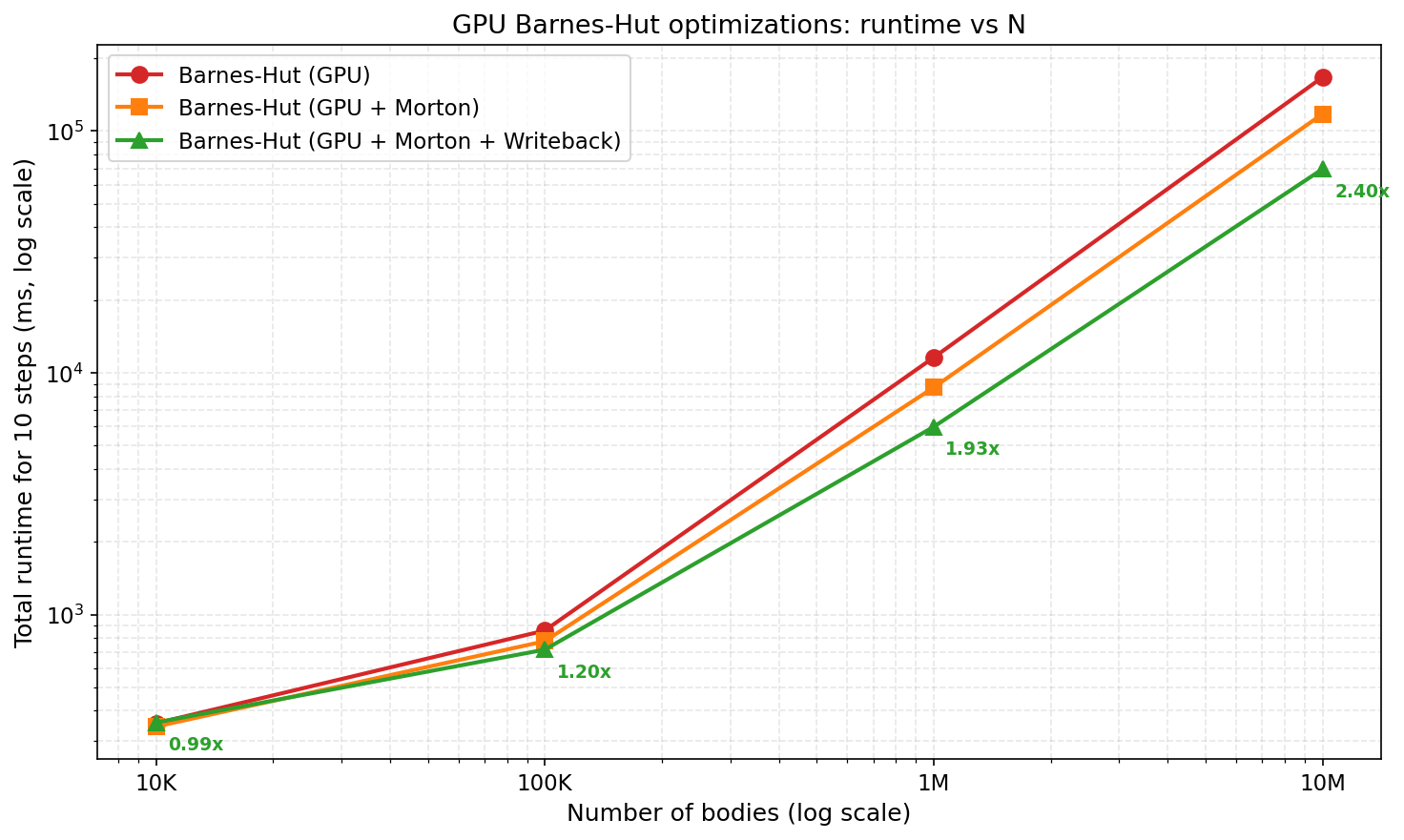
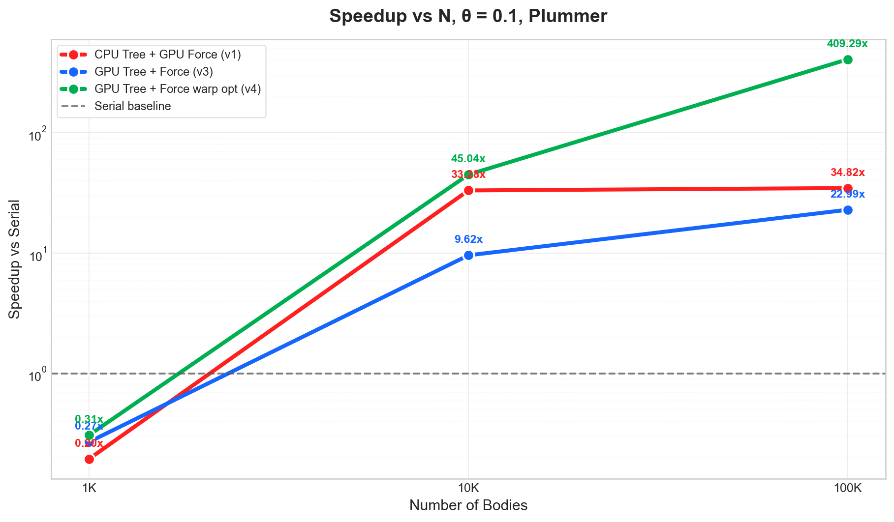
We observe that across all large enough N, v4 performs the best, with force calculation kernel now well optimized. The optimizations we performed earlier have clearly improved the numbers, as already discussed in the Nsight discussion. However, for very small number of bodies like 1k, the serial implementation on the CPU performs best, as the GPU implementations have some constant overhead in launching kernels and transferring memory between device and host, which cannot be avoided. Also, such small N does not take advantage of the thousands of threads that the GPU can and should launch to obtain maximum benefit. The graph below also showcases the same (note the log scale on the Y-axis for easier visualization).
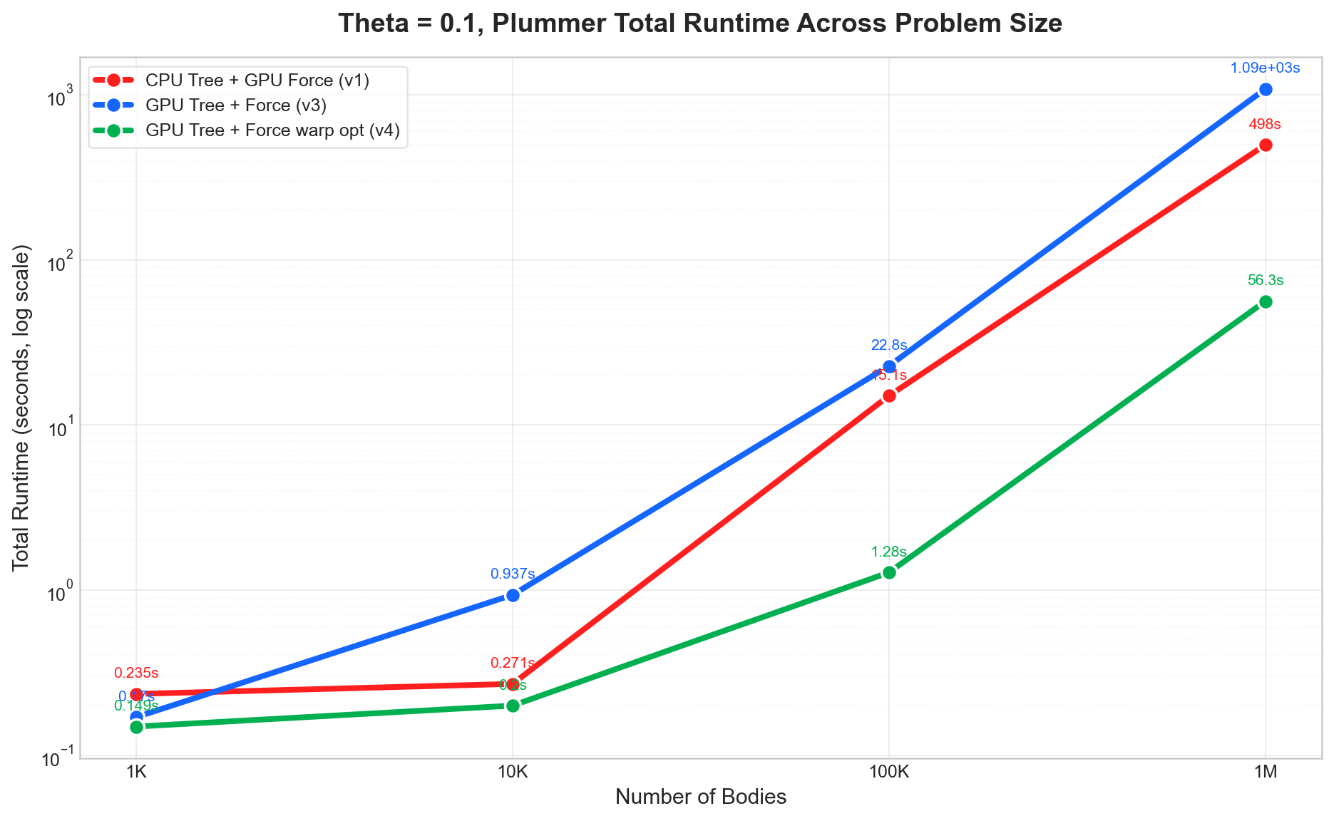
We see that the speedup over the serial implementation itself also increases as the problem size grows. This shows that while we have made optimizations and tradeoffs and tried to adapt the workload to make it more GPU-friendly through our various optimizations, there are still some overheads that can only be overcome by increasing problem size to diminish their impact. We do not plot the speedup for 1M bodies, as the serial run time is too long to measure in a reasonable amount of time.
Impact of theta on Plummer Disk, N = 100k
| Theta | Serial Total (ms) | Serial Force (ms) | v4 Total (ms) | v4 Force (ms) | v4 Speedup vs Serial |
|---|---|---|---|---|---|
| 0.1 | 525593.5 | 525480.7 | 1377.8 | 1138.5 | 381.47x |
| 0.2 | 100965.0 | 100853.0 | 607.7 | 430.2 | 166.13x |
| 0.3 | 32513.8 | 32401.9 | 384.4 | 203.5 | 84.58x |
| 0.4 | 14649.0 | 14537.1 | 252.2 | 105.2 | 58.08x |
| 0.5 | 8256.8 | 8145.2 | 224.6 | 69.2 | 36.76x |
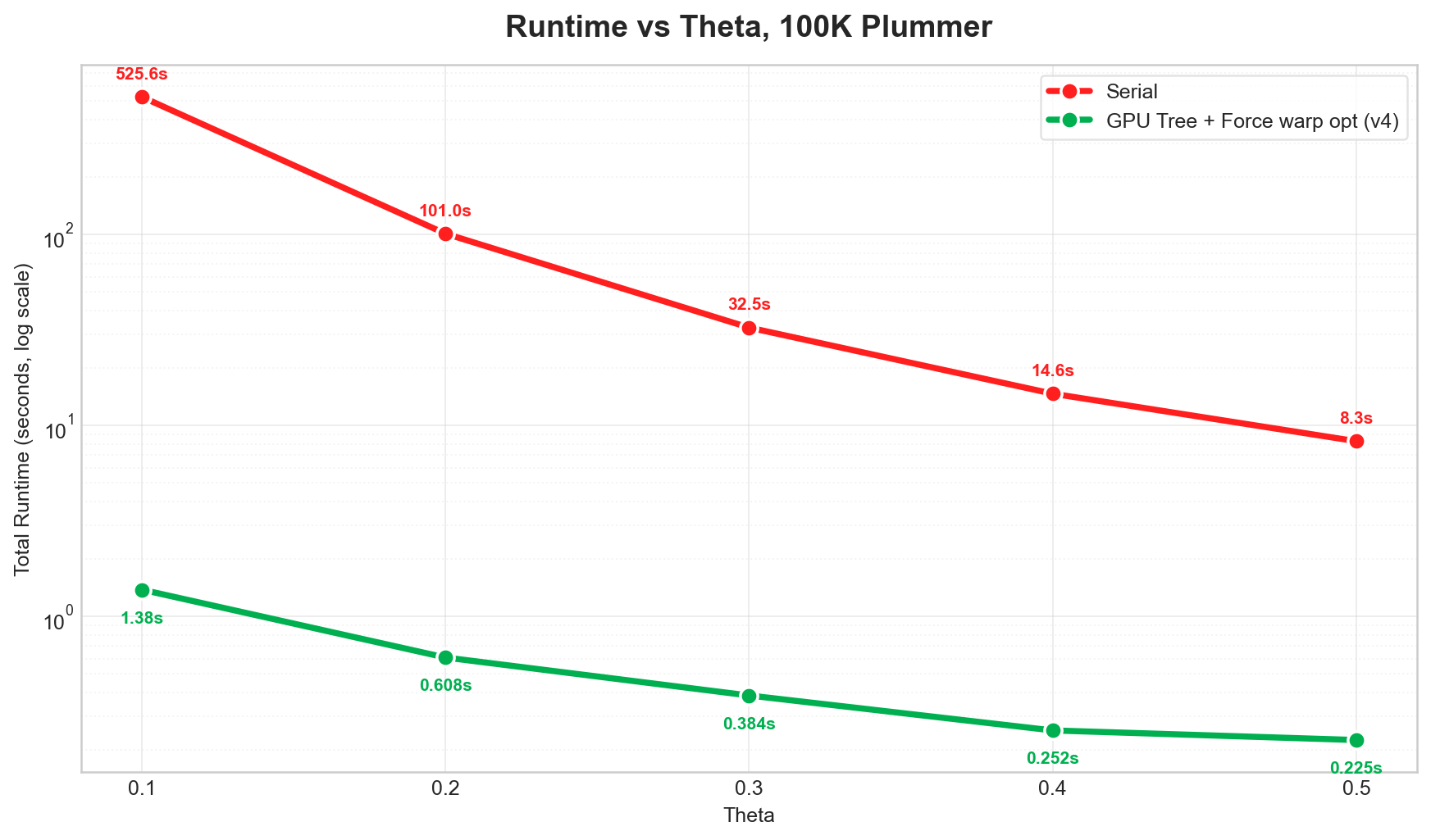
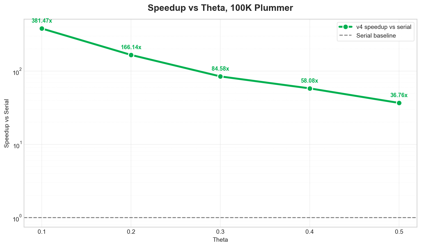
theta decides when to approximate a cluster as a point mass. Increasing theta increases the approximation rate, reducing actual work performed by the force calculations. Thus we expect that as theta increases, total runtimes should drop, and we do see that trend in both the serial and GPU implementations. We also see that the speedup of v4 over serial drops, which is again expected as the total work to be done reduces. This means lesser parallelizable work is performed, and performance gains reduce (Amdahl’s Law).
Speedup limitations:
As discussed in previous sections, our code was primarily bottlenecked by being memory-bound. We have addressed that in v4 and believe the speedups are reasonable. We note, however, that the serial overhead is quite high when running on the GPU for small N, and would like to analyze and optimize this case further. We would also like to explore other potential tree-traversal optimizations, especially the one by Liu et al 2019, to see if we can push the occupancy even higher than in v4.
GPU choice
We believe our choice of optimizing barnes-hut for the GPU was a great choice. We were able to steadily and incrementally optimize different steps of the algorithm in an orderly fashion, using performance metrics and Nsight results. Our algorithms have been written to take advantage of the large number of bodies while keeping in mind contention on shared resources. Equivalent implementations using, say, OpenMP for multithreading cannot obtain speedups as high as 400x on reasonably accessible, consumer-grade machines. It would be interesting, however, to study and understand how workloads such as Barnes-Hut can be adopted to say an FPGA.
Correctness validation
./validate runs naive O(N^2) and Barnes–Hut on identical initial conditions and compares per-body final state. All v3 results have very high accuracy:
| Run | Max position error | Max velocity error |
|---|---|---|
| 2K bodies, 20 steps, GPU v3 | 0.000% | 0.027% |
| 2K bodies, 100 steps, GPU v3 | 0.002% | 0.060% |
| 8K bodies, 20 steps, GPU v3 | 0.000% | 0.018% |
| 2K bodies, 20 steps, CPU Barnes–Hut (reference) | 0.000% | 0.030% |
We also ensure that energy and momentum are conserved across the simulation (law of conservation of energy/momentum).
In brief
We believe we have been fairly successful in optimizing our problem. We have shown that we can achieve significant speedups by moving the heaviest parts of Barnes-Hut to GPU with reasonable optimization efforts. While our original timeline included adaptive time stepping, the difficulty of optimizing the tree construction and tree walk itself consumed most of our time, barely leaving any time for the report and poster. We thus leave the implementation and optimization of adaptive time-stepping for future work.
Acknowledgements
Thank you to the Professors and TAs (and other staff involved) in ensuring this course was a great success. We truly learnt a lot from it, and the hard work has definitely helped ingrain the core ideas much better. We hope to take these ideas to wherever we go next and apply and share them so everyone writes better, faster code.
References
[1] A hierarchical O(N log N) force-calculation algorithm, Josh Barnes, Piet Hut 1986
[2] An Efficient CUDA Implementation of the Tree-Based Barnes Hut n-Body Algorithm, Martin Burtscher, Keshav Pingali 2011
[3] Maximizing Parallelism in the Construction of BVHs, Octrees, and k-d Trees, Tero Karras 2012
[4] Fast BVH Construction on GPUs, C. Lauterbach, M. Garland, S. Sengupta, D. Luebke, D. Manocha 2009
[5] Efficient GPU tree walks for effective distributed n-body simulations, Jianqiao Liu, Michael Robson, Thomas Quinn, and Milind Kulkarni 2019
Work distribution
We both split the work almost evenly, across different stages of the code writing, simulations and analysis. In particular, Dhruv and Andrew both worked on serial implementations of Barnes-Hut to get intuition of the algorithm. Dhruv worked extensively on v1, while Andrew worked on v2. We worked together to optimize v3, v4. We have split our workloads for the report and poster, handling different parts of the report and image creation in a 50-50 manner.
AI usage statement
We have used AI (Claude Opus 4.5/4.7) to help create the website (HTML). We have also used it to write the Python scripts which help us create inputs to the simulator (Plummer-disk, colliding galaxies), and to visualize our galaxy simulation outputs and convert them into gifs. For both of these use cases, we gave detailed prompts regarding the expected galaxy distributions we wanted to achieve, including some details about how the galaxies should collide. We reviewed the produced code and verified that the Physics matches that on public sources like Wikipedia. It has also been used to some extent in writing bash/Python scripts to run test cases that we provided for bench marking.