Lecture 1: Introduction and Basics
====
author: 94-842
date: August 30, 2016
font-family: Garamond
autosize: false
width:1920
height:1080
What are we trying to accomplish?
====
Here's a sample analysis.
> The analysis was shown only in class and is not viewable in this version of the notes.
Agenda
========================================================
- Course overview
- Introduction to R, RStudio and R Markdown
- Programming basics
How this class will work
========================================================
- No programming knowledge presumed
- Some stats knowledge presumed. E.g.:
- Hypothesis testing (t-tests, confidence intervals)
- Linear regression
- Class attendance is mandatory
- Class will be _very_ cumulative
Mechanics
========================================================
- Two 80 minute lectures a week:
- First 60-70 minutes: concepts, methods, examples
- Last 10-20 minutes: short labs
- Class participation (15%)
- Weekly homework (40%)
- Final project (2.5 weeks) (45%)
- **Disclaimer:** To pass the class, you must achieve a passing score on the final project (at least 23 / 45)
Mechanics
===
- __Class participation__ (15%)
- **Quizzes**: 2-3 quizzes in the second half of term. Dates TBA.
- **Labs**: Each lecture has an accompanying lab assignment.
- Course website shows how participation grade will be calculated
- __Homework assignments__ (40%)
- There will be 5 weekly HW assignments
- Single _lowest_ HW score will be dropped
- HW due at the start of class (1:30pm)
- Late homework __will not be accepted for credit__
- __Final project__ (45%)
- You will write a report analysing a policy question using a publicly available data set
Course resources
========================================================
- Assignments, office hours, class notes, grading policies, useful references on R:
http://www.andrew.cmu.edu/~achoulde/94842/
- Blackboard for __gradebook__ and for __turning in homework__
- Piazza for __forum__
- Please __post class/homework related question on Piazza__ instead of emailing the teaching staff
- Check the class website for everything else
- No required textbook, but several are _highly recommended_:
- Phil Spector, _Data Manipulation with R_
- Paul Teetor, _The R Cookbook_
- Winston Chang, _The R Graphics Cookbook_
- Norman Matloff, _The Art of R Programming: A Tour of Statistical Software Design_
Goal of this class
=====
> This class will teach you to use R to:
- Generate graphical and tabular data summaries
- Perform statistical analyses (e.g., hypothesis testing, regression modeling)
- Produce _reproducible_ statistical reports using R Markdown
- Integrate R with other tools (e.g., databases, web, etc.)
Why R?
=====
- Free (open-source)
- Programming language (not point-and-click)
- Excellent graphics
- Offers broadest range of statistical tools
- Easy to generate reproducible reports
- Easy to integrate with other tools
The R Console
====
left:30
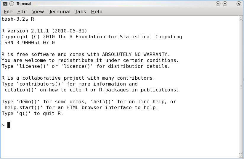
Basic interaction with R is through typing in the **console**
This is the **terminal** or **command-line** interface
***
 The R Console
====
- You type in commands, R gives back answers (or errors)
- Menus and other graphical interfaces are extras built on top of the console
- We will use **RStudio** in this class
1. Download R: http://lib.stat.cmu.edu/R/CRAN
2. Then download RStudio: http://www.rstudio.com/
======
left:30
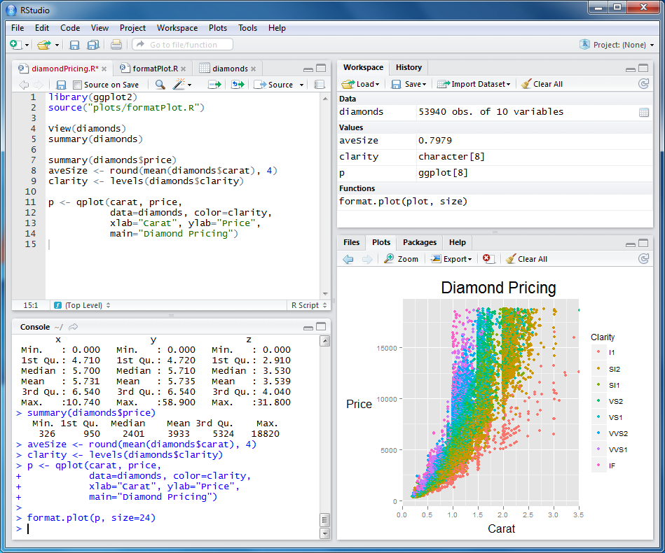
**RStudio** is an IDE for R
RStudio has 4 main windows ('panes'):
- Source
- Console
- Workspace/History
- Files/Plots/Packages/Help
***
The R Console
====
- You type in commands, R gives back answers (or errors)
- Menus and other graphical interfaces are extras built on top of the console
- We will use **RStudio** in this class
1. Download R: http://lib.stat.cmu.edu/R/CRAN
2. Then download RStudio: http://www.rstudio.com/
======
left:30
**RStudio** is an IDE for R
RStudio has 4 main windows ('panes'):
- Source
- Console
- Workspace/History
- Files/Plots/Packages/Help
***
 Console pane
========
left: 35
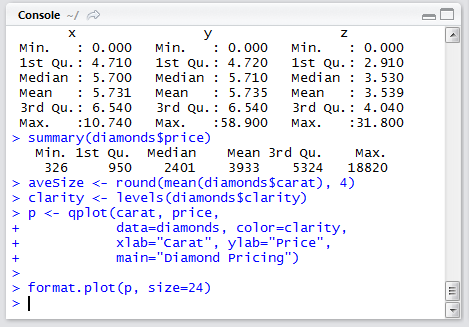
- Use the **Console** pane to type or paste commands to get output from R
- To look up the help file for a function or data set, type `?function` into the Console
- E.g., try typing in `?mean`
- Use the `tab` key to auto-complete function and object names
***
Console pane
========
left: 35
- Use the **Console** pane to type or paste commands to get output from R
- To look up the help file for a function or data set, type `?function` into the Console
- E.g., try typing in `?mean`
- Use the `tab` key to auto-complete function and object names
***
 Source pane
========
left: 35
- Use the **Source** pane to create and edit R and Rmd files
- The menu bar of this pane contains handy shortcuts for sending code to the **Console** for evaluation
***
Source pane
========
left: 35
- Use the **Source** pane to create and edit R and Rmd files
- The menu bar of this pane contains handy shortcuts for sending code to the **Console** for evaluation
***
 Files/Plots/Packages/Help pane
========
left: 35
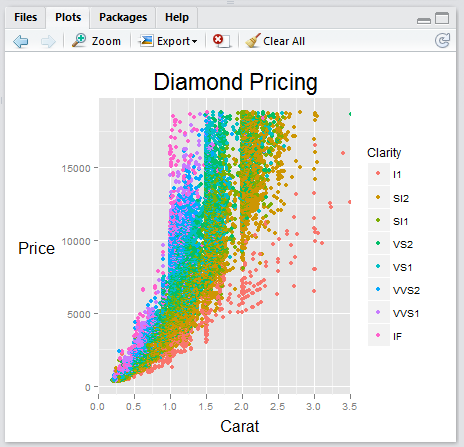
- By default, any figures you produce in R will be displayed in the **Plots** tab
- Menu bar allows you to Zoom, Export, and Navigate back to older plots
- When you request a help file (e.g., `?mean`), the documentation will appear in the **Help** tab
***
Files/Plots/Packages/Help pane
========
left: 35
- By default, any figures you produce in R will be displayed in the **Plots** tab
- Menu bar allows you to Zoom, Export, and Navigate back to older plots
- When you request a help file (e.g., `?mean`), the documentation will appear in the **Help** tab
***
 RStudio: Panes overview
========
1. __Source__ pane: create a file that you can save and run later
2. __Console__ pane: type or paste in commands to get output from R
3. __Workspace/History__ pane: see a list of variables or previous commands
4. __Files/Plots/Packages/Help__ pane: see plots, help pages, and other items in this window.
RStudio: Source and Console panes
========================================================
RStudio: Panes overview
========
1. __Source__ pane: create a file that you can save and run later
2. __Console__ pane: type or paste in commands to get output from R
3. __Workspace/History__ pane: see a list of variables or previous commands
4. __Files/Plots/Packages/Help__ pane: see plots, help pages, and other items in this window.
RStudio: Source and Console panes
========================================================
 RStudio: Console
========================================================
RStudio: Console
========================================================
 RStudio: Toolbar
=======
RStudio: Toolbar
=======
 R Markdown
====
- R Markdown allows the user to integrate R code into a report
- When data changes or code changes, so does the report
- No more need to copy-and-paste graphics, tables, or numbers
- Creates __reproducible__ reports
- Anyone who has your R Markdown (.Rmd) file and input data can re-run your analysis and get the exact same results (tables, figures, summaries)
- Can output report in HTML (default), Microsoft Word, or PDF
R Markdown
====
left: 30
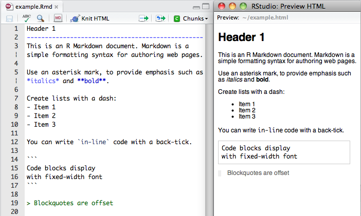
- This example shows an **R Markdown** (.Rmd) file opened in the Source pane of RStudio.
- To turn an Rmd file into a report, click the **Knit HTML** button in the Source pane menu bar
- The results will appear in a **Preview window**, as shown on the right
- You can knit into html (default), MS Word, and pdf format
- These lecture slides are also created in RStudio (R Presentation)
***
R Markdown
====
- R Markdown allows the user to integrate R code into a report
- When data changes or code changes, so does the report
- No more need to copy-and-paste graphics, tables, or numbers
- Creates __reproducible__ reports
- Anyone who has your R Markdown (.Rmd) file and input data can re-run your analysis and get the exact same results (tables, figures, summaries)
- Can output report in HTML (default), Microsoft Word, or PDF
R Markdown
====
left: 30
- This example shows an **R Markdown** (.Rmd) file opened in the Source pane of RStudio.
- To turn an Rmd file into a report, click the **Knit HTML** button in the Source pane menu bar
- The results will appear in a **Preview window**, as shown on the right
- You can knit into html (default), MS Word, and pdf format
- These lecture slides are also created in RStudio (R Presentation)
***
 R Markdown
====
left: 30
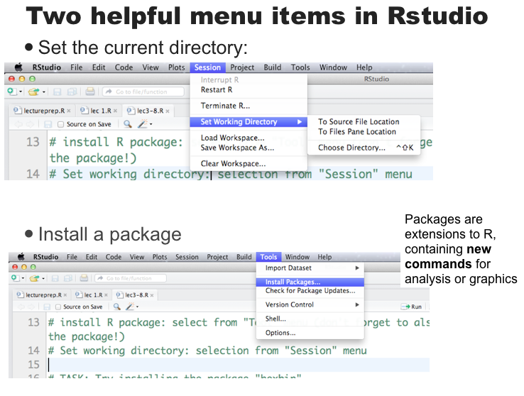
- To integrate R output into your report, you need to use R code chunks
- All of the code that appears in between the "triple back-ticks" gets executed when you Knit
***
R Markdown
====
left: 30
- To integrate R output into your report, you need to use R code chunks
- All of the code that appears in between the "triple back-ticks" gets executed when you Knit
***
 In-class exercise: Hello world!
====
1. Open **RStudio** on your machine
2. File > New File > R Markdown ...
3. Change `summary(cars)` in the first code block to `print("Hello world!")`
4. Click `Knit HTML` to produce an HTML file.
5. Save your Rmd file as `helloworld.Rmd`
> All of your Homework assignments and many of your Labs will take the form of a single Rmd file, which you will edit to include your solutions and then submit on Blackboard.
Basics: the class in a nutshell
=====
- Everything we'll do comes down to applying **functions** to **data**
- **Data**: things like 7, "seven", $7.000$, the matrix $\left[ \begin{array}{ccc} 7 & 7 & 7 \\ 7 & 7 & 7\end{array}\right]$
- **Functions**: things like $\log{}$, $+$ (two arguments), $<$ (two), $\mod{}$ (two), `mean` (one)
> A function is a machine which turns input objects (**arguments**) into an output object (**return value**), possibly with **side effects**, according to a definite rule
Data building blocks
====
You'll encounter different kinds of data types
- **Booleans** Direct binary values: `TRUE` or `FALSE` in R
- **Integers**: whole numbers (positive, negative or zero)
- **Characters** fixed-length blocks of bits, with special coding;
**strings** = sequences of characters
- **Floating point numbers**: a fraction (with a finite number of bits) times an exponent, like $1.87 \times {10}^{6}$
- **Missing or ill-defined values**: `NA`, `NaN`, etc.
Operators (functions)
====
You can use R as a very, very fancy calculator
Command | Description
--------|-------------
`+,-,*,\` | add, subtract, multiply, divide
`^` | raise to the power of
`%%` | remainder after division (ex: `8 %% 3 = 2`)
`( )` | change the order of operations
`log(), exp()` | logarithms and exponents (ex: `log(10) = 2.302`)
`sqrt()` | square root
`round()` | round to the nearest whole number (ex: `round(2.3) = 2`)
`floor(), ceiling()` | round down or round up
`abs()` | absolute value
===
```r
7 + 5 # Addition
```
```
[1] 12
```
```r
7 - 5 # Subtraction
```
```
[1] 2
```
```r
7 * 5 # Multiplication
```
```
[1] 35
```
```r
7 ^ 5 # Exponentiation
```
```
[1] 16807
```
====
```r
7 / 5 # Division
```
```
[1] 1.4
```
```r
7 %% 5 # Modulus
```
```
[1] 2
```
```r
7 %/% 5 # Integer division
```
```
[1] 1
```
Operators cont'd.
===
**Comparisons** are also binary operators; they take two objects, like numbers, and give a Boolean
```r
7 > 5
```
```
[1] TRUE
```
```r
7 < 5
```
```
[1] FALSE
```
```r
7 >= 7
```
```
[1] TRUE
```
```r
7 <= 5
```
```
[1] FALSE
```
===
```r
7 == 5
```
```
[1] FALSE
```
```r
7 != 5
```
```
[1] TRUE
```
Boolean operators
===
Basically "and" and "or":
```r
(5 > 7) & (6*7 == 42)
```
```
[1] FALSE
```
```r
(5 > 7) | (6*7 == 42)
```
```
[1] TRUE
```
(will see special doubled forms, `&&` and `||`, later)
More types
===
- `typeof()` function returns the type
- `is.`_foo_`()` functions return Booleans for whether the argument is of type _foo_
- `as.`_foo_`()` (tries to) "cast" its argument to type _foo_ --- to translate it sensibly into a _foo_-type value
**Special case**: `as.factor()` will be important later for telling R when numbers are actually encodings and not numeric values. (E.g., 1 = High school grad; 2 = College grad; 3 = Postgrad)
===
```r
typeof(7)
```
```
[1] "double"
```
```r
is.numeric(7)
```
```
[1] TRUE
```
```r
is.na(7)
```
```
[1] FALSE
```
===
```r
is.character(7)
```
```
[1] FALSE
```
```r
is.character("7")
```
```
[1] TRUE
```
```r
is.character("seven")
```
```
[1] TRUE
```
```r
is.na("seven")
```
```
[1] FALSE
```
Variables
===
We can give names to data objects; these give us **variables**
A few variables are built in:
```r
pi
```
```
[1] 3.141593
```
Variables can be arguments to functions or operators, just like constants:
```r
pi*10
```
```
[1] 31.41593
```
```r
cos(pi)
```
```
[1] -1
```
Assignment operator
===
Most variables are created with the **assignment operator**, `<-` or `=`
```r
time.factor <- 12
time.factor
```
```
[1] 12
```
```r
time.in.years = 2.5
time.in.years * time.factor
```
```
[1] 30
```
===
The assignment operator also changes values:
```r
time.in.months <- time.in.years * time.factor
time.in.months
```
```
[1] 30
```
```r
time.in.months <- 45
time.in.months
```
```
[1] 45
```
===
- Using names and variables makes code: easier to design, easier to debug, less prone to bugs, easier to improve, and easier for others to read
- Avoid "magic constants"; use named variables
- Use descriptive variable names
- Good: `num.students <- 35`
- Bad: `ns <- 35 `
The workspace
===
What names have you defined values for?
```r
ls()
```
```
[1] "time.factor" "time.in.months" "time.in.years"
```
Getting rid of variables:
```r
rm("time.in.months")
ls()
```
```
[1] "time.factor" "time.in.years"
```
First data structure: vectors
===
- Group related data values into one object, a **data structure**
- A **vector** is a sequence of values, all of the same type
- `c()` function returns a vector containing all its arguments in order
```r
students <- c("Sean", "Louisa", "Frank", "Farhad", "Li")
midterm <- c(80, 90, 93, 82, 95)
```
- Typing the variable name at the prompt causes it to display
```r
students
```
```
[1] "Sean" "Louisa" "Frank" "Farhad" "Li"
```
Indexing
====
- `vec[1]` is the first element, `vec[4]` is the 4th element of `vec`
```r
students
```
```
[1] "Sean" "Louisa" "Frank" "Farhad" "Li"
```
```r
students[4]
```
```
[1] "Farhad"
```
- `vec[-4]` is a vector containing all but the fourth element
```r
students[-4]
```
```
[1] "Sean" "Louisa" "Frank" "Li"
```
Vector arithmetic
===
Operators apply to vectors "pairwise" or "elementwise":
```r
final <- c(78, 84, 95, 82, 91) # Final exam scores
midterm # Midterm exam scores
```
```
[1] 80 90 93 82 95
```
```r
midterm + final # Sum of midterm and final scores
```
```
[1] 158 174 188 164 186
```
```r
(midterm + final)/2 # Average exam score
```
```
[1] 79 87 94 82 93
```
```r
course.grades <- 0.4*midterm + 0.6*final # Final course grade
course.grades
```
```
[1] 78.8 86.4 94.2 82.0 92.6
```
Pairwise comparisons
===
Is the final score higher than the midterm score?
```r
midterm
```
```
[1] 80 90 93 82 95
```
```r
final
```
```
[1] 78 84 95 82 91
```
```r
final > midterm
```
```
[1] FALSE FALSE TRUE FALSE FALSE
```
Boolean operators can be applied elementwise:
```r
(final < midterm) & (midterm > 80)
```
```
[1] FALSE TRUE FALSE FALSE TRUE
```
Functions on vectors
===
Command | Description
--------|------------
`sum(vec)` | sums up all the elements of `vec`
`mean(vec)` | mean of `vec`
`median(vec)` | median of `vec`
`min(vec), max(vec)` | the largest or smallest element of `vec`
`sd(vec), var(vec)` | the standard deviation and variance of `vec`
`length(vec)` | the number of elements in `vec`
`pmax(vec1, vec2), pmin(vec1, vec2)` | example: `pmax(quiz1, quiz2)` returns the higher of quiz 1 and quiz 2 for each student
`sort(vec)` | returns the `vec` in sorted order
`order(vec)` | returns the index that sorts the vector `vec`
`unique(vec)` | lists the unique elements of `vec`
`summary(vec)` | gives a five-number summary
`any(vec), all(vec)` | useful on Boolean vectors
Functions on vectors
===
```r
course.grades
```
```
[1] 78.8 86.4 94.2 82.0 92.6
```
```r
mean(course.grades) # mean grade
```
```
[1] 86.8
```
```r
median(course.grades)
```
```
[1] 86.4
```
```r
sd(course.grades) # grade standard deviation
```
```
[1] 6.625708
```
More functions on vectors
===
```r
sort(course.grades)
```
```
[1] 78.8 82.0 86.4 92.6 94.2
```
```r
max(course.grades) # highest course grade
```
```
[1] 94.2
```
```r
min(course.grades) # lowest course grade
```
```
[1] 78.8
```
Referencing elements of vectors
===
```r
students
```
```
[1] "Sean" "Louisa" "Frank" "Farhad" "Li"
```
Vector of indices:
```r
students[c(2,4)]
```
```
[1] "Louisa" "Farhad"
```
Vector of negative indices
```r
students[c(-1,-3)]
```
```
[1] "Louisa" "Farhad" "Li"
```
More referencing
===
`which()` returns the `TRUE` indexes of a Boolean vector:
```r
course.grades
```
```
[1] 78.8 86.4 94.2 82.0 92.6
```
```r
a.threshold <- 90 # A grade = 90% or higher
course.grades >= a.threshold # vector of booleans
```
```
[1] FALSE FALSE TRUE FALSE TRUE
```
```r
a.students <- which(course.grades >= a.threshold) # Applying which()
a.students
```
```
[1] 3 5
```
```r
students[a.students] # Names of A students
```
```
[1] "Frank" "Li"
```
Named components
===
You can give names to elements or components of vectors
```r
students
```
```
[1] "Sean" "Louisa" "Frank" "Farhad" "Li"
```
```r
names(course.grades) <- students # Assign names to the grades
names(course.grades)
```
```
[1] "Sean" "Louisa" "Frank" "Farhad" "Li"
```
```r
course.grades[c("Sean", "Frank","Li")] # Get final grades for 3 students
```
```
Sean Frank Li
78.8 94.2 92.6
```
Note the labels in what R prints; these are not actually part of the value
Useful RStudio tips
====
Keystroke | Description
----------|-------------
`` | autocompletes commands and filenames, and lists arguments for functions. Highly useful!
`` | cycle through previous commands in the console prompt
`` | lists history of previous commands matching an unfinished one
`` | paste current line from source window to console. Good for trying things out ideas from a source file.
`` | as mentioned, abort an unfinished command and get out of the + prompt
In-class exercise: Hello world!
====
1. Open **RStudio** on your machine
2. File > New File > R Markdown ...
3. Change `summary(cars)` in the first code block to `print("Hello world!")`
4. Click `Knit HTML` to produce an HTML file.
5. Save your Rmd file as `helloworld.Rmd`
> All of your Homework assignments and many of your Labs will take the form of a single Rmd file, which you will edit to include your solutions and then submit on Blackboard.
Basics: the class in a nutshell
=====
- Everything we'll do comes down to applying **functions** to **data**
- **Data**: things like 7, "seven", $7.000$, the matrix $\left[ \begin{array}{ccc} 7 & 7 & 7 \\ 7 & 7 & 7\end{array}\right]$
- **Functions**: things like $\log{}$, $+$ (two arguments), $<$ (two), $\mod{}$ (two), `mean` (one)
> A function is a machine which turns input objects (**arguments**) into an output object (**return value**), possibly with **side effects**, according to a definite rule
Data building blocks
====
You'll encounter different kinds of data types
- **Booleans** Direct binary values: `TRUE` or `FALSE` in R
- **Integers**: whole numbers (positive, negative or zero)
- **Characters** fixed-length blocks of bits, with special coding;
**strings** = sequences of characters
- **Floating point numbers**: a fraction (with a finite number of bits) times an exponent, like $1.87 \times {10}^{6}$
- **Missing or ill-defined values**: `NA`, `NaN`, etc.
Operators (functions)
====
You can use R as a very, very fancy calculator
Command | Description
--------|-------------
`+,-,*,\` | add, subtract, multiply, divide
`^` | raise to the power of
`%%` | remainder after division (ex: `8 %% 3 = 2`)
`( )` | change the order of operations
`log(), exp()` | logarithms and exponents (ex: `log(10) = 2.302`)
`sqrt()` | square root
`round()` | round to the nearest whole number (ex: `round(2.3) = 2`)
`floor(), ceiling()` | round down or round up
`abs()` | absolute value
===
```r
7 + 5 # Addition
```
```
[1] 12
```
```r
7 - 5 # Subtraction
```
```
[1] 2
```
```r
7 * 5 # Multiplication
```
```
[1] 35
```
```r
7 ^ 5 # Exponentiation
```
```
[1] 16807
```
====
```r
7 / 5 # Division
```
```
[1] 1.4
```
```r
7 %% 5 # Modulus
```
```
[1] 2
```
```r
7 %/% 5 # Integer division
```
```
[1] 1
```
Operators cont'd.
===
**Comparisons** are also binary operators; they take two objects, like numbers, and give a Boolean
```r
7 > 5
```
```
[1] TRUE
```
```r
7 < 5
```
```
[1] FALSE
```
```r
7 >= 7
```
```
[1] TRUE
```
```r
7 <= 5
```
```
[1] FALSE
```
===
```r
7 == 5
```
```
[1] FALSE
```
```r
7 != 5
```
```
[1] TRUE
```
Boolean operators
===
Basically "and" and "or":
```r
(5 > 7) & (6*7 == 42)
```
```
[1] FALSE
```
```r
(5 > 7) | (6*7 == 42)
```
```
[1] TRUE
```
(will see special doubled forms, `&&` and `||`, later)
More types
===
- `typeof()` function returns the type
- `is.`_foo_`()` functions return Booleans for whether the argument is of type _foo_
- `as.`_foo_`()` (tries to) "cast" its argument to type _foo_ --- to translate it sensibly into a _foo_-type value
**Special case**: `as.factor()` will be important later for telling R when numbers are actually encodings and not numeric values. (E.g., 1 = High school grad; 2 = College grad; 3 = Postgrad)
===
```r
typeof(7)
```
```
[1] "double"
```
```r
is.numeric(7)
```
```
[1] TRUE
```
```r
is.na(7)
```
```
[1] FALSE
```
===
```r
is.character(7)
```
```
[1] FALSE
```
```r
is.character("7")
```
```
[1] TRUE
```
```r
is.character("seven")
```
```
[1] TRUE
```
```r
is.na("seven")
```
```
[1] FALSE
```
Variables
===
We can give names to data objects; these give us **variables**
A few variables are built in:
```r
pi
```
```
[1] 3.141593
```
Variables can be arguments to functions or operators, just like constants:
```r
pi*10
```
```
[1] 31.41593
```
```r
cos(pi)
```
```
[1] -1
```
Assignment operator
===
Most variables are created with the **assignment operator**, `<-` or `=`
```r
time.factor <- 12
time.factor
```
```
[1] 12
```
```r
time.in.years = 2.5
time.in.years * time.factor
```
```
[1] 30
```
===
The assignment operator also changes values:
```r
time.in.months <- time.in.years * time.factor
time.in.months
```
```
[1] 30
```
```r
time.in.months <- 45
time.in.months
```
```
[1] 45
```
===
- Using names and variables makes code: easier to design, easier to debug, less prone to bugs, easier to improve, and easier for others to read
- Avoid "magic constants"; use named variables
- Use descriptive variable names
- Good: `num.students <- 35`
- Bad: `ns <- 35 `
The workspace
===
What names have you defined values for?
```r
ls()
```
```
[1] "time.factor" "time.in.months" "time.in.years"
```
Getting rid of variables:
```r
rm("time.in.months")
ls()
```
```
[1] "time.factor" "time.in.years"
```
First data structure: vectors
===
- Group related data values into one object, a **data structure**
- A **vector** is a sequence of values, all of the same type
- `c()` function returns a vector containing all its arguments in order
```r
students <- c("Sean", "Louisa", "Frank", "Farhad", "Li")
midterm <- c(80, 90, 93, 82, 95)
```
- Typing the variable name at the prompt causes it to display
```r
students
```
```
[1] "Sean" "Louisa" "Frank" "Farhad" "Li"
```
Indexing
====
- `vec[1]` is the first element, `vec[4]` is the 4th element of `vec`
```r
students
```
```
[1] "Sean" "Louisa" "Frank" "Farhad" "Li"
```
```r
students[4]
```
```
[1] "Farhad"
```
- `vec[-4]` is a vector containing all but the fourth element
```r
students[-4]
```
```
[1] "Sean" "Louisa" "Frank" "Li"
```
Vector arithmetic
===
Operators apply to vectors "pairwise" or "elementwise":
```r
final <- c(78, 84, 95, 82, 91) # Final exam scores
midterm # Midterm exam scores
```
```
[1] 80 90 93 82 95
```
```r
midterm + final # Sum of midterm and final scores
```
```
[1] 158 174 188 164 186
```
```r
(midterm + final)/2 # Average exam score
```
```
[1] 79 87 94 82 93
```
```r
course.grades <- 0.4*midterm + 0.6*final # Final course grade
course.grades
```
```
[1] 78.8 86.4 94.2 82.0 92.6
```
Pairwise comparisons
===
Is the final score higher than the midterm score?
```r
midterm
```
```
[1] 80 90 93 82 95
```
```r
final
```
```
[1] 78 84 95 82 91
```
```r
final > midterm
```
```
[1] FALSE FALSE TRUE FALSE FALSE
```
Boolean operators can be applied elementwise:
```r
(final < midterm) & (midterm > 80)
```
```
[1] FALSE TRUE FALSE FALSE TRUE
```
Functions on vectors
===
Command | Description
--------|------------
`sum(vec)` | sums up all the elements of `vec`
`mean(vec)` | mean of `vec`
`median(vec)` | median of `vec`
`min(vec), max(vec)` | the largest or smallest element of `vec`
`sd(vec), var(vec)` | the standard deviation and variance of `vec`
`length(vec)` | the number of elements in `vec`
`pmax(vec1, vec2), pmin(vec1, vec2)` | example: `pmax(quiz1, quiz2)` returns the higher of quiz 1 and quiz 2 for each student
`sort(vec)` | returns the `vec` in sorted order
`order(vec)` | returns the index that sorts the vector `vec`
`unique(vec)` | lists the unique elements of `vec`
`summary(vec)` | gives a five-number summary
`any(vec), all(vec)` | useful on Boolean vectors
Functions on vectors
===
```r
course.grades
```
```
[1] 78.8 86.4 94.2 82.0 92.6
```
```r
mean(course.grades) # mean grade
```
```
[1] 86.8
```
```r
median(course.grades)
```
```
[1] 86.4
```
```r
sd(course.grades) # grade standard deviation
```
```
[1] 6.625708
```
More functions on vectors
===
```r
sort(course.grades)
```
```
[1] 78.8 82.0 86.4 92.6 94.2
```
```r
max(course.grades) # highest course grade
```
```
[1] 94.2
```
```r
min(course.grades) # lowest course grade
```
```
[1] 78.8
```
Referencing elements of vectors
===
```r
students
```
```
[1] "Sean" "Louisa" "Frank" "Farhad" "Li"
```
Vector of indices:
```r
students[c(2,4)]
```
```
[1] "Louisa" "Farhad"
```
Vector of negative indices
```r
students[c(-1,-3)]
```
```
[1] "Louisa" "Farhad" "Li"
```
More referencing
===
`which()` returns the `TRUE` indexes of a Boolean vector:
```r
course.grades
```
```
[1] 78.8 86.4 94.2 82.0 92.6
```
```r
a.threshold <- 90 # A grade = 90% or higher
course.grades >= a.threshold # vector of booleans
```
```
[1] FALSE FALSE TRUE FALSE TRUE
```
```r
a.students <- which(course.grades >= a.threshold) # Applying which()
a.students
```
```
[1] 3 5
```
```r
students[a.students] # Names of A students
```
```
[1] "Frank" "Li"
```
Named components
===
You can give names to elements or components of vectors
```r
students
```
```
[1] "Sean" "Louisa" "Frank" "Farhad" "Li"
```
```r
names(course.grades) <- students # Assign names to the grades
names(course.grades)
```
```
[1] "Sean" "Louisa" "Frank" "Farhad" "Li"
```
```r
course.grades[c("Sean", "Frank","Li")] # Get final grades for 3 students
```
```
Sean Frank Li
78.8 94.2 92.6
```
Note the labels in what R prints; these are not actually part of the value
Useful RStudio tips
====
Keystroke | Description
----------|-------------
`` | autocompletes commands and filenames, and lists arguments for functions. Highly useful!
`` | cycle through previous commands in the console prompt
`` | lists history of previous commands matching an unfinished one
`` | paste current line from source window to console. Good for trying things out ideas from a source file.
`` | as mentioned, abort an unfinished command and get out of the + prompt
**Lab 1**: http://www.andrew.cmu.edu/~achoulde/94842/
- Look under Tenatative Schedule Tue 08/30 or on Blackboard
- Submit modified .Rmd file on Blackboard