Empirical Research Methods II
Spring 2000
Lab 5
Due: Tuesday, April 4th.
1 FTP, Course Data Sets, and Turning in the Assignment
The data sets we will be using for the course are all stored in:
/afs/andrew.cmu.edu/course/88/241/data
1) Go to the Programs menu under Start (bottom left of the screen). Find and select Command Prompt.
2)
At the
prompt inside the Command Prompt window, change directories to c:\temp, a local
directory you can write to while you are on the machine in this cluster, by
typing: cd c:\temp
3)
Now
invoke ftp by typing: ftp unix.andrew.cmu.edu (see Error!
Reference source not found.). Login with your andrew id and
password.
4)
Change
directories on the andrew side by typing:
cd
/afs/andrew.cmu.edu/course/88/241/data
5) Go into binary mode by typing: bin
6) Get the file lab5qs.doc by typing: get lab5qs.doc
7) Type: get learning.mtp
8) Type: get comp.mtp
9) Type: get vote.mtp
Turning In Assignments
1. Open MS Word (not in ftp, but rather from the Start menu), and open the file you just downloaded: lab5qs.doc, which should be sitting in the c:\temp directory.
2. In Word, fill in your name and email id, and then go to the File menu, choose "Save As", and name the file <your-email-id>-lab5.doc. E.g., since my email address is scheines@andrew.cmu.edu, my file name would be: scheines-lab5.doc
You can copy Minitab results and graphs into this file, and turn it in electronically at any time before the beginning of the next class. To turn in your file electronically, use ftp in binary mode and deposit the file in the /afs/andrew/course/88/241/handin directory. If you already have ftp running, follow steps 4, 5 and 6 below. To do it from scratch, follow all of these steps:
1. Open command prompt
2. Cd
into the directory in which your Word file resides (e.g., c:\temp)
3. type
ftp
unix.andrew.cmu.edu
4. To
enter binary transfer mode, type: bin
5. To
change the remote target directory,
type: cd
/afs/andrew.cmu.edu/course/88/241/handin
6. To transfer the file, type: put <file-name>
You cannot overwrite your Word file once it is turned in, so make sure it is finished before you transfer it over. Uri will send you email with the grade on your lab.
Keep a copy of your file, in case the transfer fails or it somehow
gets corrupted.
2 Correlation between X and e and Bias
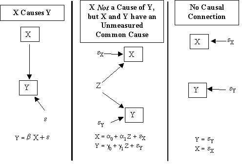
We have discussed at length how correlation between X and e can arise and how this can bias b1 (the estimate of b1) away from 0 even when b1 is actually 0, that is, X has no effect at all on Y. For example, in lab 3 we showed how the first two causal structures in Figure 1 are indistinguishable, and will both result in estimates of b1 that are non-zero.

Now we concentrate on how a correlation between X and e biases the size of the estimated relationship between X and Y even when X is a cause of Y. Consider a problem in which X is exposure to lead (Lead) and Y is IQ-score (IQ).

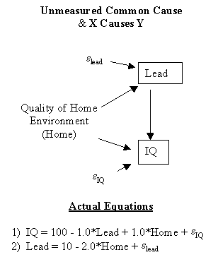
In Figure 2, we show the causal process relating IQ and Lead. IQ is caused by Lead, the Quality of the Home Environment (an unmeasured cause that we abbreviate as Home), and eIQ, the other unmeasured causes of IQ which are assumed to be independent of Lead and Home. Furthermore, Lead is also caused by Home and other unmeasured causes, eLead, which are assumed to be independent of Home.
The actual equation relating IQ to its causes, Lead, Home, and eIQ, is
1) IQ = 100 – 1.0*Lead + 1.0*Home +eIQ.
The coefficient on Lead equals –1.0. This is a causal coefficient, which indicates that a 1 unit increase in Lead exposure causes a 1 point drop in IQ holding constant Home and the other causes of IQ. The equation also indicates that a 1 unit increase in Home causes a 1 unit increase in IQ, holding everything else constant.
The actual equation relating Lead to its causes, Home and eLead, is
2) Lead = 10 –
2.0*Home + eLead
This indicates that a 1
unit increase in Home causes a 2 unit decrease in Lead, holding everything else
constant.
Even though this system involves many variables, suppose that data are only available on IQ and Lead. Suppose these data are used to estimate a bivariate regression relating IQ to Lead. To better understand the regression that will be estimated, notice that equation 1 can be rewritten as equation 3:
3) IQ = 100 –1.0*Lead + e,
where e = Home + eIQ. In the typical regression, the disturbance term is assumed to be independent of the predictor variable. In equation 3, however, IQ is expressed as a function of Lead and a disturbance e, which is not independent of Lead. Just like in the Unmeasured Common Cause process in question 1, one of the unmeasured causes of IQ, Home, is also a cause of Lead. This means that the disturbance term e in equation 3, which is the sum of Home and eIQ, is correlated with Lead.
The purpose of this exercise is to explore how this correlation biases the estimated coefficient on Lead in a bivariate regression relating IQ to Lead. A bias occurs if the estimated coefficient differs from the true causal coefficient, even when we have an infinite sample. In this case, the true causal coefficient relating IQ to Lead is –1.0, which represents the effect of a 1 unit change in Lead on IQ assuming all other causes of IQ are held constant.
Open the file misspec3.mtp. In this file there is a sample of size 1000 on Lead and IQ.
Question 2a: In the bivariate regression relating IQ to Lead, think about the correlation between Lead and the disturbance term e, which is actually a composite of Home and eiq. Do you think the correlation between Lead and e is positive, negative, or zero? Explain.
Question 2b: Given your answer to question 2a, how would you expect the coefficient estimate of Lead in the bivariate regression relating IQ to Lead to differ from –1.0? Would you expect the coefficient estimate on Lead to be less than, greater than, or equal to -1.0, that is, would you expect the bias to be negative, positive, or 0?
Question 2c. Estimate a regression in which IQ is the dependent variable and Lead the independent variable and report the regression output in your Word file. Is your estimated coefficient on Lead greater than, less than, or equal to –1.0? What would this mean for policy--do you underestimate or overestimate the harmful effects of Lead on IQ?
Question 2d. Is there anything in the regression relating IQ and Lead that would suggest that the regression model you estimated is misspecified—i.e., the unmeasured causes of IQ are correlated with Lead? For example, does the scatterplot of the residuals against the fitted values indicate any departure from the all-clear plot in Hamilton? Is there any other diagnosis you might do that might reveal your model is misspecified?
3 Controlling for Omitted Common Causes
In exercise 2, we had you estimate a bivariate regression relating IQ to Lead because those were the only measured variables available. The exercise was meant to show you how the unmeasured common cause Home led to an estimate of the coefficent relating Lead to IQ that was different from -1.0, the causal coefficient.
Open the file misspec4.mtp. In this file there is a sample of size 1000 on Lead, IQ, and Home.
Question 3a: First, estimate a bivariate regression relating IQ to Lead. Based on the coefficient estimate of Lead, which is biased, would you reject at the .01 level of significance the null hypothesis that the coefficient equals -1.0 (the true causal coefficient) versus the alternative that the coefficient does not equal -1.0? Recall that in minitab - the normal t-test is computed for a null hypothesis in which the coefficient under test is assumed to equal 0. Nevertheless - you can perform the same test by seeing if the null hypothesis falls outside of the 99% confidence interval around the computed estimate.
Question 3b: What regression should you compute to get an unbiased estimate of the true effect of Lead on IQ? Do this regression, and report the results. Based on the coefficient estimate of Lead in this regression, would you reject at the .01 level of significance the null hypothesis that the coefficient equals -1.0 versus the alternative that the coefficient does not equal -1.0?
Question 3c. Did you reach a different conclusion regarding the null hypothesis from the regressions you computed in 1a and 1b? If so, why?
4 Simulating Data
Open a new worksheet in Minitab. In this problem we want you to first simulate data from a known model - and then compute regression estimates with alternative specifications.

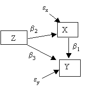
4a. Suppose that all relations are linear. Convert the model in Figure 3 into a set of equations. Type the equations into your Word File. Now pick numerical values for the coefficients. For example, you might choose b1 = -.7. Write down the equations with numerical values instead of coefficients.
4b. To generate data, you must pick distributions for the exogenous variables, that is, the variables that are only causes and not effects. Figure out which variables are exogenous, and write down distributions for them. For example, writing: A ~ N(0,4) specifies that variable a is distributed as Normal with mean = 0 and standard deviation = 4.
4c. Using your exogenous variables and numerical equations in the answers to 5b and 5a, generate 2000 cases of data in minitab for all the variables in Figure 3. When you are done, perform a regression in which Y is the dependent variable and X the independent. How does the estimate b1 compare to the value you chose for b1. If it differs, explain why.
4d. Do a hypothesis test of whether b1 = the value you chose for it in 5a. Explain how you did it, and report the results in your Word file.
5e. Repeat 5d, but this time do a multiple regression in which Y is the dependent variable and X and Z the independent variables. Explain how these results differed from those you got in 5d, and why.