Empirical Research Methods II
Spring 2000
Lab 4
Due: Tuesday, March 21st
1) FTP, Course Data Sets, & Turning in Assignments
2) Shipbuilding
3) Unions and Company Sales
4) Voter Fraud
1 FTP, Course Data Sets, and Turning in Assignments
The data sets we will be using for the course are all stored in:
/afs/andrew.cmu.edu/course/88/241/data
So the first thing we will do is use ftp to download a file from this directory.
Figure 1. Calling FTP within a Command Prompt
1) Go to the Programs menu under Start (bottom left of the screen). Find and select Command Prompt.
2)
At the
prompt inside the Command Prompt window, change directories to c:\temp, a local
directory you can write to while you are on the machine in this cluster, by
typing: cd c:\temp
3)
Now
invoke ftp by typing: ftp unix.andrew.cmu.edu (see Figure
1). Login with your andrew id and password.
4)
Change
directories on the andrew side by typing:
cd
/afs/andrew.cmu.edu/course/88/241/data
5) Go into binary mode by typing: bin
6) Get the file lab4qs.doc by typing: get lab4qs.doc
7) Type: get learning.mtp
8) Type: get comp.mtp
9) Type: get vote.mtp
Turning In Assignments
Lab assignments should be turned in as MS Word files. To make things easier on everyone, we want you to answer the questions for this lab by inserting your answers into an MS Word file that already has the questions, then by saving it with the appropriate name, and finally turning it in via ftp as you have already been doing. To do this:
1. Open MS Word (not in ftp, but rather from the Start menu), and open the file you just downloaded: lab4qs.doc, which should be sitting in the c:\temp directory.
2. In Word, fill in your name and email id, and then go to the File menu, choose "Save As", and name the file <your-email-id>-lab4.doc. E.g., since my email address is scheines@andrew.cmu.edu, my file name would be: scheines-lab4.doc
You can copy Minitab results and graphs into this file, and
turn it in electronically at any time before the beginning of the next
class. To turn in your file
electronically, use ftp in binary mode and deposit the file in the /afs/andrew/course/88/241/handin directory.
If you already have ftp running, follow steps 4, 5 and 6 below. To do it from scratch, follow all of these
steps:
1. Open command prompt
2. Cd
into the directory in which your Word file resides (e.g., c:\temp)
3. type
ftp
unix.andrew.cmu.edu
4. To
enter binary transfer mode, type: bin
5. To
change the remote target directory,
type: cd
/afs/andrew.cmu.edu/course/88/241/handin
6. To transfer the file, type: put <file-name>
You cannot overwrite your Word file once it is turned in, so make sure it is finished before you transfer it over. Uri will send you email with the grade on your lab.
Keep a copy of your file, in case the transfer fails or it somehow
gets corrupted.
2 Learning to Build Ships
Go to the File Menu, and then use Open Worksheet to open the file ‘learning.mtp’.
During World War II, the U.S. built ships on an unprecedented scale. Beginning in 1941, the U.S. commenced building a new type of ship, the Liberty Ship. As time progressed, the number of manhours required to build a Liberty ship fell sharply. There have been a number of theories as to the causes of this drop in manhours per ship (mps). On one view, called the “learning” theory, the more time a shipbuilding yard engages in production, the more efficient it becomes at ship building. That is, the mps falls with the total time since production began. On another view, called the “economy of scale view,” efficency depends just on the scale of production. That is, the more ships produced in a time period, the lower the mps in that time period.
The data set records the following three variables for each of the 42 months the ships were produced, with the observations ordered in time.
Output Number of ships produced in the month
MPS Average manhours per ship produced in the month
Month The number of months since production started
Question 2a. What is the dependent variable (effect) corresponding to each theory? Write the answer in your Word file for this and all of the questions below.
Question 2b. For the learning theory, what variable would you construct or use as the cause, or independent variable?
Question 2c. For the economy of scale theory, what variable would you construct or use as the cause, or independent variable?
Question 2d. Perform regressions to evaluate both theories. Report the results in your Word file, and describe the scientific conclusion these results suggest.
Question 2e. In both theories, the effect is not necessarily a linear function of the cause. You can use regression diagnostics to locate certain problems in regression, among them non-linearity. One of the most powerful regression diagnositcs is the residual vs. fits plot.[1] To produce this plot in Minitab, do Stat à Regression à Regression, and in the dialog box click on the Graphs button. This will produce a dialog box as we show in Figure 2. Make sure the Residuals vs. fits is checked, and then click OK, and then do the regression.
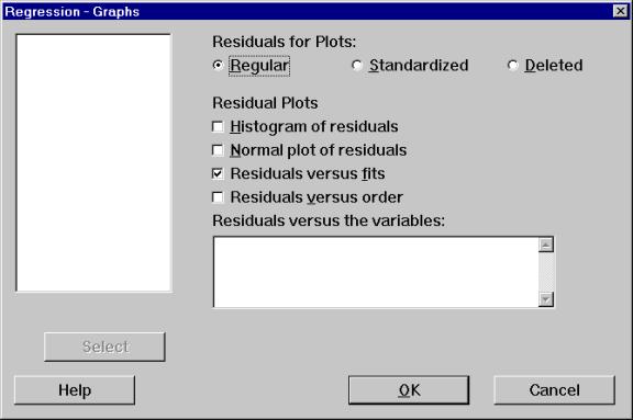
What problems, if any, do the residual vs. fits plots uncover?
Question 2f. One way to fix non-linearity is to transform the independent variables. Create new independent variables that are the natural logs of your original independent variables. Do the regressions again, and again examine the residual vs. fits plots, and again describe what you found.
Question 2g. Now that you have done all of these statistical analyses, what scientific conclusion do you come to? Which theory fits the data better? Report and explain your results in your Word file.
3 Unions and Company Sales
Open the file comp.mtp in Minitab. This file contains data on sales for each of 36 quarters, spanning 1980 to 1988, of a company in two different markets, as well as the total sales of all similar companies in those markets. The variables are as follows:
MarLA Total Market sales in LA (in $100,000s)
CompLA Company’s sales in LA market (in $1,000s)
MarCol Total Market sales in Columbus (in $100,000s)
CompCol Company’s sales in Columbus market (in $1,000s)
Quarter 1-36, starting in the first quarter of 1980.
Both markets involved big and small contracts. Firms that bid on big contracts were required to use unionized labor, whereas any firm could bid on small jobs. The company employed unionized labor in both markets, and specialized in large jobs that took several years to complete. The company and its union became embroiled in a dispute that eventually caused the union to strike in the 2nd quarter of 1986 in LA (quarter 26 in comp.mtp), and the 2nd quarter of 1987 in Columbus (quarter 30). The company hired scabs to replace the unionized labor, which prevented it from competing for large jobs. According to the company, this caused its sales to be less than they would have been had the union not struck. Further, the company claimed that it couldn’t realistically compete for large jobs as early as a full year before the strike because the dispute had been made public and firms that employed them were loath to award them contracts for fear that their labor dispute would prevent the work from being completed successfully. The union, of course, denies the company’s causal assertions. According to them, the company was able to do enough additional small jobs to maintain its sales.
Suppose you are hired as a consultant to determine whether the data support the company or the union perspective. For each of the questions below, record a few sentences and supporting analyses in your Word file.
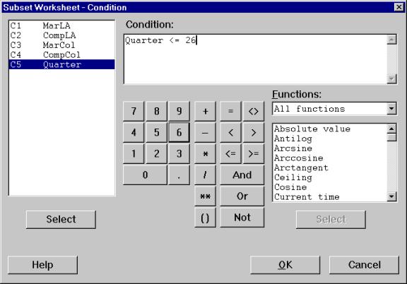
Question 3a. The company claimed its sales after the strike were less than they would have been if the union had not struck. In both markets, the overall market sales increased, and the company felt that in the absence of the strike, its sales would have increased proportionally. Examine whether the company’s sales before the strikes were related to the overall market sales, both in Columbus and LA. To do this, you can create a new worksheet that contains only the data before the LA strike, and another for Columbus. Use the Manip à Subset Worksheet command. It will ask you to subset by which rows to include, and when you click OK, you will get a dialogue box like the one in Figure 3 below. Use the boolean expresseion Quarter <= 26 for the LA strike, and <= 30 for the Columbus strike.
Question 3b. The union claimed that the company “maintained its sales,” despite the strike. According to the union, the average sales of the company after the strike were the same as before the strike. Examine this claim for both cities using a dummy-variable regression. To do this for LA, for example, you need to create a dummy-variable that is equal to 0 before the strike in LA and equal to 1 after the strike. Do this as follows:
- Calc à
Calculator
- Fill in the Calculator Dialog box as we show in Figure 4.
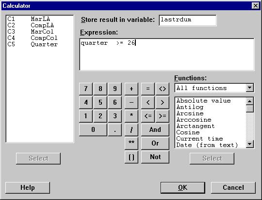
This will create a variable called “lastridum” in C6, which equals 1 for quarters 26-36, and 0 otherwise. Now do a regression to answer the question for LA. Do the analogous analysis for Columbus, keeping in mind that the date of the strike was different for the two cities.
Question 3c. The company claimed that its sales would have increased proportionally with the market, but didn’t as a result of the strike. If this were true, then the company’s market share, i.e., the ratio of company sales to overall market sales, would have been lower after the strikes. Examine this claim for both cities using a dummy-variable regression.
Question 3d. Both the union and the company acknowledged that any effect from the strike would have been manifested as early as a year before the actual strike. Reconsider questions a, b, and c, assuming that the dispute would have had an effect a year before the actual strike.
Question 3e. The union admits that there was a decline in the company’s market share after the labor dispute, but claims that the decline took place long before this, and that this fact undermines the causal claims of the company. Using analyses similar to the ones you have already been employing, examine and evaluate this claim with the data.
4 Voter Fraud
In 1993 in Philadelpia there was a special election to fill a State Senate vacancy. On voting machines, the Republican candidate, Bruce Marks, received 19,691 votes compared to 19,127 votes for the Democratic candidate, William Stinson. In contrast, Stinson got 1,396 absentee votes versus 371 for Marks, giving him an overall victory. The Republicans cried foul. Among other charges, they claimed that homeless people were hired to recruit absentee votes for Stinson. A judge ruled that the absentee votes had been improperly collected and awarded the seat to the Republican candidate Marks. The decision was appealed, and you are brought in to help settle the issue scientifically.
In the file, voter.mtp, you have data on 22 State Senate elections from Philadelphia between 1982 to 1993. The variables are:
Year Year of the election
District District
Demabs Number of absentee ballots cast for the Dem. candidate
Repabs Number of absentee ballots cast for the Rep. candidate
Dempop Number of machine ballots cast for the Dem. candidate
Reppop Number of machine ballots cast for the Rep. candidate
The last election, number 22, is the election under dispute. In rough terms, your task is to examine whether the absentee ballots cast in this election are extraordinary.
Question 4a. The judge remarks that election 22 seems odd in that the machine vote was close but the absentee vote was not. The judge reasons that the machine vote is a reasonable measure of the sentiments of the population, and that the absentee ballot ought to reflect roughly the same sentiments. Using only the prior 21 elections, analyze whether the difference between the Democratic and Republican absentee votes is linearly related to the difference between the Democratic and Republican machine votes. This will require several steps, some to manipulate the data and some to perform statistical analyses. Whereas in the past we have guided you step-by-step, here we are setting you a little more on your own. Document the variables you used in your analysis, explain your choice of statistical tools, and report the results in your Word file.
Question 4b. Based on your analysis in part a and the machine vote in the contested election, what is your best guess as to the difference between Democratic and Republican absentee votes in the contested election? Explain the basis for your guess.
Question 4c. After hearing your best guess, the judge asks what would be a plausible range of values for the difference between Democratic and Republican absentee votes in the contested election, given the difference in Democratic and Republican machine votes in the contested election. You can construct a confidence interval for a predicted value of the dependent variable in a regression model, called a ‘Prediction Interval.’ Follow these steps to do so:
- Stat à Regression à Regression
- Click on the ‘Options’ button in the Regression Dialog Box
- In the Options Dialog Box, type in the value of the independent (predictor) variable in the box titled: ‘Prediction Intervals for new observations.’ For example, if you were predicting the value of Y given a value of X = 25, then you would type 25 in this box. After typing the value you want, click OK.
- Click OK in the Regression Dialog Box.
The output of the calculation is in the Session window. You will see two intervals, one labeled 95%CI and the other 95%PI. You want PI. In your Word file, report the prediction interval for the difference between Democratic and Republican absentee votes in the contested election, given the difference between Democratic and Republican machine votes for the election. Does the actual difference between Democratic and Republican absentee votes in the contested election fall within this interval?
Question 4d. The judge does not want his ruling overturned by the higher court, so he instructs you to be very conservative in your statistical analysis. He wants to be 99% confident that the difference between Democratic and Republican absentee votes in the contested election is not the result of chance. Does the actual difference between Democratic and Republican absentee votes in the contested election fall within the interval corresponding to the 99% confidence level?
Question 4e. The judge is worried that in doing your analysis you built a model upon data that did not include the contested election. Would your findings in questions c and d change if you included the contested election in the regressions you estimated in all previous questions? Report your results and explain.