Empirical Research Methods II
Spring 2000
Lab 3:
Bivariate Regression 2
Due: Tuesday, March 14th
1) FTP, Course Data Sets, & Turning in Assignments
2) Misspecification
3) R2 and Coefficient Significance
4) Connecticut Crackdown
1 FTP, Course Data Sets, and Turning in Assignments
The data sets we will be using for the course are all stored in:
/afs/andrew.cmu.edu/course/88/241/data
So the first thing we will do is use ftp to download a file from this directory.
Figure 1. Calling FTP within a Command Prompt
1) Go to the Programs menu under Start (bottom left of the screen). Find and select Command Prompt.
2)
At the
prompt inside the Command Prompt window, change directories to c:\temp, a local
directory you can write to while you are on the machine in this cluster, by
typing: cd c:\temp
3)
Now
invoke ftp by typing: ftp unix.andrew.cmu.edu (see Figure
1). Login with your andrew id and password.
4)
Change
directories on the andrew side by typing:
cd
/afs/andrew.cmu.edu/course/88/241/data
5) Go into binary mode by typing: bin
6) Get the file lab3qs.doc by typing: get lab3qs.doc
7) Get the file c-signif.mtp by typing: get c-signif.mtp
8) Get the file crackdown.mtp by typing: get crackdown.mtp
9) Get the file misspec2.mtp by typing: get misspec2.mtp
10)
Don't quit ftp
Turning In Assignments
Lab assignments should be turned in as MS Word files. To make things easier on everyone, we want you to answer the questions for this lab by inserting your answers into an MS Word file that already has the questions, then by saving it with the appropriate name, and finally turning it in via ftp as you have already been doing. To do this:
1. Open MS Word (not in ftp, but rather from the Start menu), and open the file you just downloaded: lab3qs.doc, which should be sitting in the c:\temp directory.
2. In Word, fill in your name and email id, and then go to the File menu, choose "Save As", and name the file <your-email-id>-lab3.doc. E.g., since my email address is scheines@andrew.cmu.edu, my file name would be: scheines-lab3.doc
You can copy Minitab results and graphs into this file, and
turn it in electronically at any time before the beginning of the next
class. To turn in your file
electronically, use ftp in binary mode and deposit the file in the /afs/andrew/course/88/241/handin directory.
If you already have ftp running, follow steps 4, 5 and 6 below. To do it from scratch, follow all of these
steps:
1. Open command prompt
2. Cd
into the directory in which your Word file resides (e.g., c:\temp)
3. type
ftp
unix.andrew.cmu.edu
4. To
enter binary transfer mode, type: bin
5. To
change the remote target directory,
type: cd
/afs/andrew.cmu.edu/course/88/241/handin
6. To transfer the file, type: put <file-name>
You cannot overwrite your Word file once it is turned in, so make sure it is finished before you transfer it over. Uri will send you email with the grade on your lab.
Keep a copy of your file, in case the transfer fails or it somehow
gets corrupted.
2. Misspecification
The purpose of this exercise is to give you a hands on feel for the effect of a common type of misspecification you need to worry about when you are doing bivariate regression.
Open the file misspec2.mtp in Minitab. The file contains 1000 rows of simulated data on six variables: x1,y1, x2,y2, x3, and y3. For each pair of variables: <x1,y1>, < x2,y2>, and < x3,y3>, exactly one of the three causal processes in Figure 2 applies. Your job is to match which process created which data.
Figure 2. Three Generating Structures
Each of these graphs contains a path diagram of the causal structure, as well as the corresponding equations.
In the first process, X Causes Y, X is a cause of Y. The regression relating Y and X is
Y = b0 + b1X + e,
where e
is a disturbance term representing all other unmeasured causes of Y, which are
assumed to be independent of X. This is
the model that is assumed to be truly producing the data on Y on X that we have
been considering.
In the second process, which we abbreviate as Unmeasured Common Cause, X is not a cause of Y, but X and Y have a common unmeasured cause, Z. The common cause Z makes the "disturbance term" for Y, which is composed of Z and the other unmeasured causes of Y (eY), to be correlated with X. X and Y are also affected by other causes that are independent of Z. The relationships are:
Y = g0 + g1Z + ey
X = a0 + a1Z + ex,
where ey and ex represent the other causes of Y and X, which are independent of Z (ey and ex are also independent of each other, reflecting that Y and X share only one cause, Z).
In the third process, No Causal Connection, X is not a cause of Y and there is no unmeasured common cause of X and Y--i.e., the unmeasured causes of X, ex, are independent of the unmeasured causes of Y, ey. This process is represented by
Y = ey
X = ex,
where ey and ex are independent.
You have a sample of size 1,000 on <x1,y1>,
a sample of 1,000 on < x2,y2>, and a sample of
1,000 on <x3,y3>.
One of these samples was drawn from the the X causes Y process, one
from the Unmeasured Common Cause process,
and one from the No Causal Connection process.
Question 2a. In a sample from the X causes Y process, would you expect X and Y to be correlated? Explain. In a sample from the Unmeasured Common Cause process, would you expect X and Y to be correlated? Explain. In a sample from the No Causal Connection process, would you expect X and Y to be correlated? Explain.
Question 2b. Estimate the following three bivariate regressions and report the coefficient estimates, standard errors, T-statistics, and R2 :
1. Make y1 the dependent variable and x1 the independent variable.
2. Make y2 the dependent variable and x2 the independent variable.
3. Make y3 the dependent variable and x3 the independent variable.
Question 2c. Using the results of your regressions, take your best guess as to the which pairs came from which processes. That is, fill in the following table as best you can.
Fill in the blanks with either:
X Causes Y
Unmeasured Common Cause
No Causal Connection
Data on < x1,y1> were produced by the ____________________ process.
Data on < x2,y2> were produced by the ____________________ process.
Data on < x3,y3> were produced by the ____________________ process.
3. R2 and
coefficient significance
The purpose of this exercise is to give you some hands on feel for the factors that contribute to the significance of coefficient estimates in a linear regression.
Open the file c-signif.mtp in Minitab. The file contains simulated data on four variables: x1,y1,x2, and y2.
In the underlying process that generated these data, x1 was a cause of y1, and x2 a cause of y2. Both y1 and y2 had other causes, e1 and e2, that were independent of x1 and x2 respectively. Both y1 and y2 were generated according to the following linear equations, in which the intercept is zero, and the slopes are b1 and b2 respectively:
y1 = b1x1 + e1
y2 = b2x2 + e2
First, do a scatterplot of x1 and y1, and then another of x2 and y2.
Question 3a. Based on the two scatterplots, what is your guess about the relative size of b1 and b2, the slope coefficients? That is, do you think that b1 is less than or greater than b2? Record your answer in this and all subsequent questions in your Word file for this lab.
Question 3b. Based on the two scatterplots, what is your guess about the relative size of the R2 of the two regressions?
Question 3c. Based on the two scatterplots, what is your guess about the relative size of the T-statistic of the estimates of b1 and b2? Relatedly, what is your guess about the relative sizes of the p-values associated with these coefficient estimates?
Question 3d. Based on the two scatterplots, which slope coefficient estimate do you think is more likely to be significantly different from zero at the .05 level?
Question 3e. Use Minitab to estimate the two regressions. Now compare the estimated values to the predictions you made in questions a, b, c, and d. If your predictions for questions 3c and 3d were wrong, what might you have overlooked?
4. The Connecticut
Speeding Crackdown
Open the file crackdown.mtp. In this file there is a sample of nine years listing the year and the number of traffic fatalities in that year:
Year 1951-1959
Fatalites Number of deaths from traffic accidents that year
Plot the fatalities versus year as follows:
1)
Graph ® Plot
2) In the Plot Dialog Box (Figure 3), insert Fatalities in the Y column and Year in the X column and then change the Display from Symbol to Connect. This will connect the points in the plot, helping you see patterns that might exist in time ordered data.
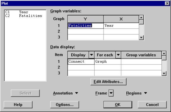
Figure 3. Plot Dialog Box
Question 4a. From your plot, what year stands out as unusual?
Question 4b. The crackdown occurred at the end of 1955 and took effect, if at all, starting in 1956. Based on your plot, does it appear that the crackdown was effective in reducing traffic fatalities?
Question 4c. First, create a dummy-variable that is equal to 0 before the crackdown and equal to 1 after the crackdown. Do this as follows:
- Calc à
Calculator
- Fill in the Calculator Dialog box as we show in Error! Reference source not found..
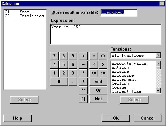
Figure 4
This will create a variable called “crackdown” in C3, which equals 1 for years 1956-59-36, and 0 otherwise. Now compute a dumy-variable regression to test whether the crackdown reduced the annual number of traffic fatalities beginning in 1956. Report the results of the regression in your Word file. Using a .05 significance level, would you accept or reject the null hypothesis that the crackdown had no effect on the number of fatalities versus the alternative that the crackdown permanently reduced the number of traffic fatalities?
Question 4d. The Governor is up for reelection and immediately fires his first statistician, who did the regression in question 3c and simply stopped there. He informs you that the big jump in traffic fatalities in 1955 signaled a permanent change in the environment that began at the start of 1955. He argues that this change would have resulted in much higher number of fatalities in every subsequent year beginning with 1956 had it not been for the crackdown. What dummy variable would you create to represent a permanent change in the background level of traffic danger at the start of 1955?