Analysis of Experiment 3

Setup of Experiment 3

--Points on Level 1: (1,120), (2,90), (3,65), (4,45), (5,30), (6,18), (7,11), (8,6), (9,3), (10,2.50), (11,2.25)

--Points on higher levels: Multiples of level 1 points—e.g., (3,360), (6,270) on Level 3

Optimal Choices

Round	Income	Price of X	QX:QY	Level	QX
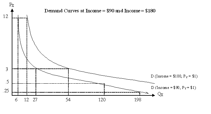
1	90	3	9:3	3	27
2	180	12	6:18	2	12
3	90	0.5	10:2.5	12	120
4	30	3	9:3	1	9
5	90	0.25	11:2.25	18	198
6	180	3	9:3	6	54
7	90	12	6:18	1	6

Analysis: WTP Schedule

Point on Level 1 (QX:QY)	WTPX (in units of Y)
1:120	--
2:90	30
3:65	25
4:45	20
5:30	15
6:18	12
7:11	7
8:6	5
9:3	3
10:2.5	0.5
11:2.25	0.25

--Optimal Choice: Q_X:Q_Y such that WTP_X(Q_X:Q_Y) = P_X/P_Y = P_X

--Maximum Level = Income/(Cost of chosen Q_X:Q_Y), e.g., in Round 1, P_X = $3, cost of 9:3 = 3 x 9 + 1 x 3 = $30, so level = $90/$30 = 3

--Optimal Q_X = Level x Q_X in optimal choice, e.g., in Round 1, Q_X = 3 (for Level 3) x 9 (from 9:3) = 27

Elasticities of Demand

Price elasticity of demand

E_D = -%ΔQ_D / %ΔP = -[(Q₁ – Q₀)/Q₀] / [(P₁ – P₀)/P₀]

For example, Income = $90, P₀ = $3, Q₀ = 27 (Round 1), Income = $90, price falls to P₁ = $0.50, quantity rises to Q₁ = 120 (Round 3)

E_D = -[(120 – 27)/27] / [(0.50 – 3)/3] = 3.44/0.83 = 4.14

Income elasticity of demand

E_I = %ΔQ_D / %ΔI = [(Q₁ – Q₀)/Q₀] / [(I₁ – I₀)/I₀]

For example, Income I₀ = $90, P = $3, Q₀ = 27 (Round 1), income rises to I₁ = $180, P = $3, quantity rises to Q₁ = 54 (Round 6)

E_I = [(54 – 27)/27] / [(180 – 90)/90] = 2/2 = 1