Fluid #2: Flow Around A
Baseball USING FLOTRAN
Introduction:
In this example you
will model air flow over a baseball.
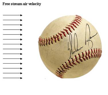
Physical Problem:
Compute and plot
the velocity distribution over the baseball shown below.
Problem Description:
·
A
Baseball is 7.48 cm in diameter. (radius of 3.74cm)
·
The
flow velocity (of air) over the baseball is approximately 40 m/s.
·
Objective:
To
plot the velocity profile around the ball.
To
graph the velocity distribution above and below the ball.
·
You are
required to hand in print outs for the above.
·
Figure:
IMPORTANT:
Convert all
dimensions and forces into SI units.
·
Create
the larger area, then the area defining the baseball.
·
Subtract the baseball area from the larger area.
·
Define
the Element Properties as a 2D Air Element
·
Define
the Material Properties of the Air Element (Density and Viscosity
are the important qualities)
 |
Mesh the plate with a mesh size of 0.005 on the edges of the
baseball, and 0.2 on the edges of the outer area.
|
|
Apply Boundary Conditions (No Slip along the edges of the baseball,
velocity along the left line of the large area, and Atmospheric
Pressure (P=0 in ANSYS) along the top, right and bottom lines of the
large area. |
|
Iterate 20 times and solve. (Ideally the iteration count would be at
least several thousand times to make sure that the solution converges…
but computational time dictates that in order to be able to solve the
problem in a reasonable amount of time, the iteration number should be
trimmed down to 20)
|
|
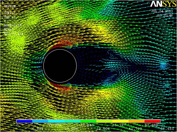
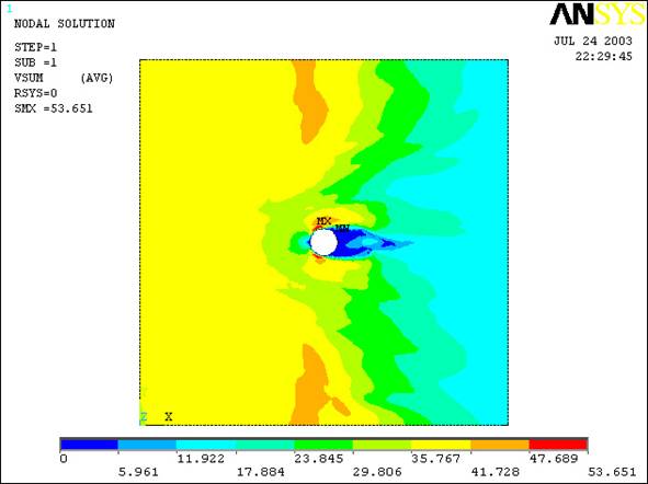
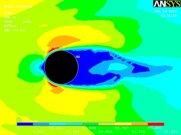
Plot the Velocity
distribution in the X and Y directions, this is the answer you should
obtain with 20 iterations: |
(Contour Plot)
(Vector Plot)