24-451 Feedback Controls
Fall 2000
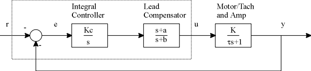
In this lab, you will use a lead compensator to improve on the performance of the motor speed controllers used in Labs 2 and 3. An integrator in the controller will be used to remove steady-state error and reject disturbances, and the lead compensator will be used to improve settling time. A block diagram showing the closed-loop system is shown below.
The controller in this diagram consists of three parts: an integrator/summer , a lead compensator, and a variable gain. This will require the use of three op amps rather than the two used in the last lab. The lead compensator pole (p) and zero (z), and the variable controller gain (Kc) will be designed to meet settling time and percent overshoot requirements. You will perform this design with the aid of Matlab. The closed loop step, ramp, and frequency responses will be examined, as well as properties of the controller.
The motor, amplifier, and tach together represent the plant in this lab. The open loop TF is of the same form as that in Labs 1,2 and 3, i.e.
![]()
You can compute the plant's gain and time constant from the open-loop step response, just as was done in the previous labs. Or you can simply use the motor that you used in the previous lab. Since you should now be familiar with the identification procedure used in the previous labs, the details of the procedure are not included here. For more details, bring one of the previous lab handouts. However, a brief outline of the procedure is included below.
| Connect Power Supply to Amplifier | |||||
| Connect Motor and Tach to Amplifier, Oscilloscope and Function Generator | |||||
Set the function generator and oscilloscope.
| |||||
| Measure Step Response, Obtain K and |
In this section, you will add the integral controller and lead compensator. The controller uses three op-amps from the LM324 quad op-amp chip. The circuit is shown below. Notice that since there are three op-amps, and each one inverts, the negatives result in a negative feedback (which is what we want) and a negative on the input (which we don't want). This is not a problem since we can simply invert one of the signals when viewing them on the oscilloscope to get the proper sign. The sign of the feedback term depends on which way the tach wires are connected.
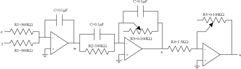
The left op-amp in the circuit is an inverting summer/integrator. The input/output relationship for this portion of the circuit is:
![]()
The center op-amp is the lead compensator. It's transfer function is:
![]()
Given the capacitor value(s) the pole is determined by R3 (a potentiometer used as a variable resistor between 0 and 100K Ohms) and the zero is determined by R2, another potentiometer. You will compute the values of R2 and R3 to give the desired response based on the root locus.
The right op-amp is an adjustable inverting gain. R5 is a potentiometer which is adjustable between 0 and 100K Ohms. The input/output relationship for this portion of the circuit is:
![]()
These three circuits together provide the inverting adjustable integral controller and lead compensator represented by the dotted box in the block diagram. It's transfer function (ignoring the extra negative sign) is:
![]()
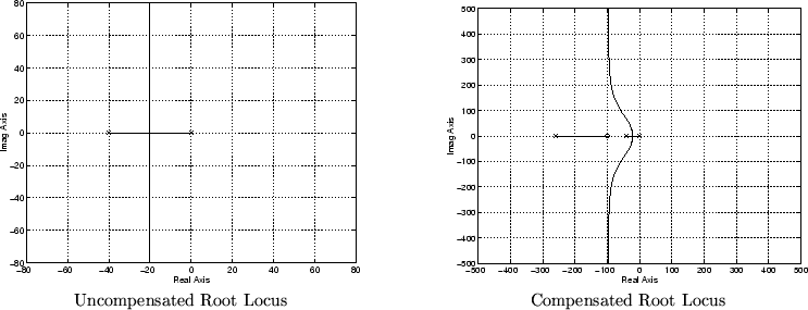
The lead compensator helps speed the response of the system by moving the closed-loop poles to the left. Without the lead compensator, the root locus has a vertical asymptote halfway between the integrator (s=0) and the open loop pole (as shown below). Therefore, the the fastest the system can respond in closed-loop would be half as fast as in open loop (with better error and disturbance rejection of course) which will not be fast enough to meet the specifications.
After placing a pole and a zero on the negative real axis before closing the loop, there will still be a vertical asymptote (#p-#z=2) but the position of the asymptote can be changed. The asymptote will be at:
So the asymptote will be shifted by (b-a)/2. Therefore, if you place the compensator pole further to the left than the zero (but both further to the left than the motor pole) you can ``bend'' the root locus to the left as shown below.
You will choose the lead compensator pole (-b) and zero (-a), as well as the controller gain (Kc) to meet the following response specifications:
| S.S. Error to a step = 0 | |
| %OV = 16.3% | |
| Ts = 0.04s |
You will use MATLAB to make the calculations using the root locus. The basic procedure is, that after placing the zero (-a) you will find the pole (-b) to make the root locus go through a desired point. Then you will find the gain using rlocfind. You will then calculate the appropriate resistor values to give you the appropriate gains and positions. The root locus is a plot of all possible closed-loop pole locations as the gain, Kc is varied. MATLAB cannot draw the root locus until particular positions for the pole and zero are chosen. This is an iterative process, so you will have to calculate the appropriate values, plot the root locus, and see how well it worked.
| Define the variables numo and deno to be the numerator and denominator polynomials of the open-loop transfer function, including the 1/s in the controller (but not Kc, and not the lead compensator).\ | |
| Define numl and denl to be the numerator and denominator of the lead compensator with a and b as obtained previously. | |
| Type num=conv(numo,numl) and den=conv(deno,denl) to multiply the compensator transfer function by the plant transfer function. | |
| Type rlocus(num,den). The root locus, similar to the previously shown compensated root locus will be drawn. Print it out. (Be sure to label it appropriately) |
![]()
The values of C, R1, and R4 are shown in the circuit diagram.
| Be sure the power is turned off. | |
| Connect the GND terminal of the amplifier to the GND post on the breadboard with a banana cable. | |
| Connect the GND post to the top row of the breadboard with a small jumper wire. | |
| Connect the top row of the breadboard to the second column in from the right with a small jumper. This is the GND column. | |
| Use a long wire to connect the -V terminal of the amplifier to the rightmost column of the breadboard. This is the -V column. | |
| Use a long wire to connect the +V terminal of the amplifier to the first column to the left of the right half section of the breadboard. |
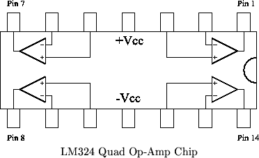
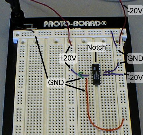
| Insert the chip in the center of the right half of the breadboard so that it straddles the small gap in the middle with the end with the notch facing up (see picture). | |
| Connect the +Vcc pin of the chip (pin 4) to the +V column with a small jumper. | |
| Connect the -Vcc pin of the chip (pin 11) to the -V column with a small jumper. | |
| Connect the + input pins of two of the op-amps (pins 12 and 5 in the picture) to the GND column with jumpers. This sets the zero reference voltage for the first and third op-amps. | |
| Connect the + input pin (pin 3) of the second op-amp to that of a third op amp (pin 5) with a short jumper. This grounds the third op-amp. |
Circuit Power Connections
| Connect a | |
| Attach two 560K resistors (green-blue-yellow) between the negative input of the first op-amp (pin 13) and two different free rows of the breadboard. These free resistor ends will be referred to as the controller inputs. |
| Connect a | |
| Set 100K potentiometer to the value for R2. Connect it between these same two free rows (in parallel with the capacitor.) | |
| Connect one end of these two components to the output of the first op-amp (pin 14) with a jumper. | |
| Connect the other end of these two components to the negative input of the second op-amp (pin 2). | |
| Connect another | |
| Set the resistance of a potentiometer to the value you computed for R3. Connect it between the same output and negative input pins you just connected the capacitor between. |
| Set the resistance of a second potentiometer to the value you computed for R5. Connect it between the output of the third op-amp (pin 7) and the corresponding negative input (pin 6). | |
| Connect a 1.5K resistor between the negative input of the third op-amp (pin 6) and the output of the second op-amp (pin 1). |
| Detach the red clip from the IN terminal of the amplifier (this should be the signal from the function generator) and attach it to the free end of one of the controller input resistors in the op-amp circuit. This is r, the reference input. | |
| Detach the red clip from the tachometer signal wire. Attach both the clip and the wire to the free end of the other controller input resistor. This is the feedback signal, -y. | |
| Connect a wire between the output pin of the third op-amp (pin 7) and the IN terminal of the amplifier. This is the control signal, u. |
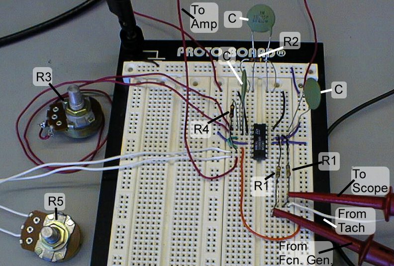
Complete Controller Circuit (Note R2 is simply a resistor in this photo.)
| Check your connections. It is particularly important that the power be applied to the op-amp in the right direction, and that none of the pins on the chip are shorted to each other. Be careful that none of the resistor or capacitor leads touch each other. | |||||||||
| Set the function generator to a square input of amplitude 1V, offset 1V, and frequency 1Hz. This will be a square wave alternating between 1V and 3V. | |||||||||
| Set the trigger to source 1 at a level of 2V with upward slope. | |||||||||
| Set both voltage scales on the oscilloscope to 1V/div. | |||||||||
| Set the time scale to 10ms/div, and the horizontal delay to 40ms. | |||||||||
| Adjust the vertical position of traces 1 and 2 so that the origin of each is exactly at the center of the screen. | |||||||||
| Set trace 2 to invert mode. This will get rid of the negative sign when viewing the signal. | |||||||||
| Turn on the power. If the voltage levels on the power supply do not go up to 20V, then turn it off immediately since something is most likely shorted. If this is the case check your connections. | |||||||||
| If the motor spins uncontrollably, you are in positive feedback. If this is the case, interchange the two leads from the tachometer. | |||||||||
| Measure the error by using the math function on the oscilloscope. To do this, press the +/- button, turn the math function on, select menu, and choose the ``-'' function. Set units/div=1V and offset=3V using the knob normally used for cursors. | |||||||||
Use the cursors to measure the following:
| |||||||||
| Print this screen. |
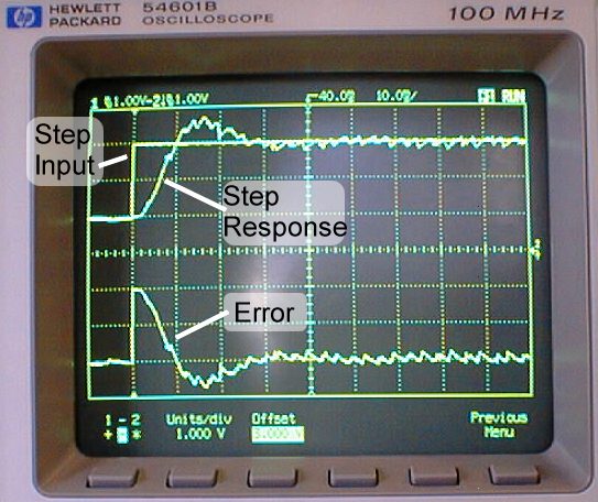
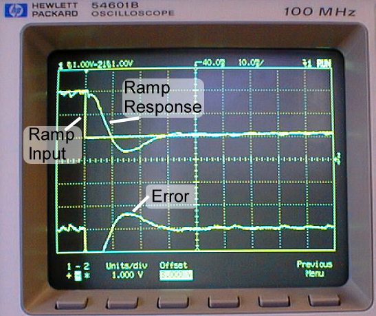
| Step Response | Ramp Response |
The writeup due date will be announced in class. Only one writeup is required per group. A formal format is not required, but be sure to address the following issues. Include all your work in the writeup and justify all your answers. Tabulate results wherever appropriate.
Lab 4 - Motor Speed Control with Lead Compensator and Integral Control
This document was generated using the LaTeX2HTML translator Version 96.1 (Feb 5, 1996) Copyright © 1993, 1994, 1995, 1996, Nikos Drakos, Computer Based Learning Unit, University of Leeds.
The command line arguments were:
latex2html -no_reuse -split 0 lab4.tex.
The translation was initiated by Jonathan E Luntz on Wed Apr 30 12:07:22 EDT 1997
And redone by Ajay Juneja on Tue
Apr 20 14:16:25 EST 1999
![]()