Assignment 2
Ziyin Xiong / ziyinx
1. Exploring loss functions
1.1 Fitting a voxel grid
Loss: binary cross-entropy on logits (F.binary_cross_entropy_with_logits). Left: optimised source; right: target.

1.2 Fitting a point cloud
Loss: symmetric Chamfer distance written from scratch with knn_points(K=1): mean squared distance from every source point to its nearest target point plus the reverse direction. Left: optimised source; right: target.

1.3 Fitting a mesh
Loss: Chamfer on 5000 surface samples + 0.1 × uniform Laplacian smoothing (‖vi − mean of neighbours‖, averaged over vertices). Left: optimised source; right: target.

2.1 Image to voxel grid
Decoder. fc 512 → 256×23, then four ConvTranspose3d(k4,s2,p1)+BN+ReLU blocks (2→4→8→16→32) and a 3×3×3 conv to one logit channel; output bias initialised to logit(0.1), the approximate occupancy prior. Loss: BCE on logits.
Training. ResNet18 encoder (ImageNet-pretrained, fine-tuned), Adam lr 4e-4, batch 32, 10000 iterations.
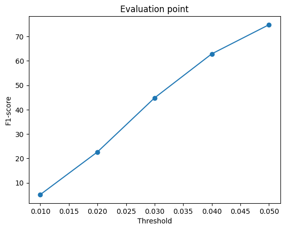
F1@0.05 = 57.77 on the 678 test chairs.

columns: input | prediction | GT mesh | GT voxels


2.2 Image to point cloud
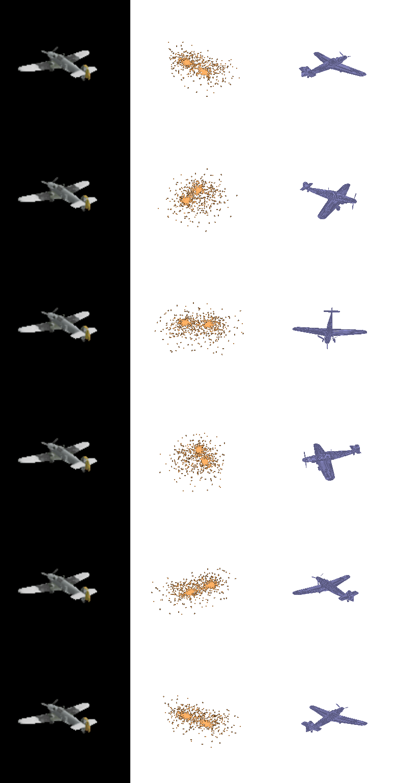
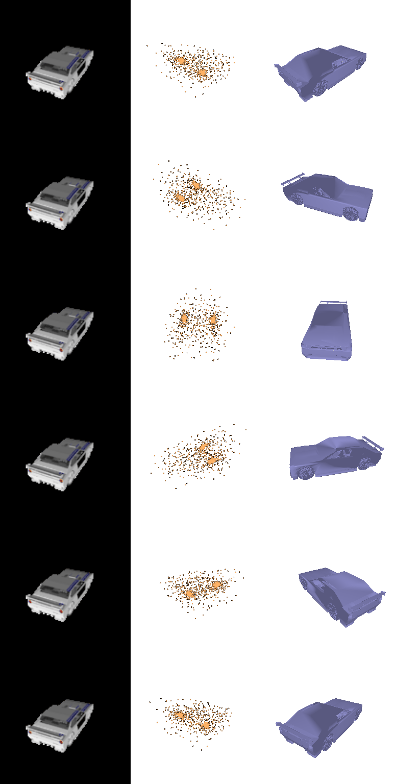
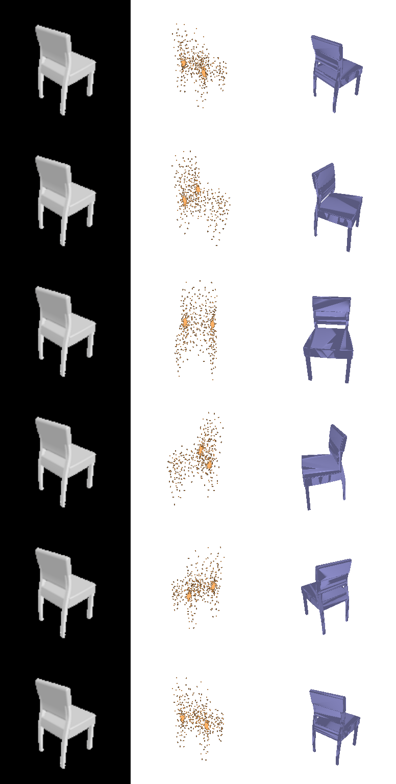
Decoder. MLP 512→1024→2048→4096→3N (LeakyReLU, tanh output), N = 1000 points. Loss: symmetric Chamfer against 1000 points sampled from the GT mesh.
Training. ResNet18 encoder (ImageNet-pretrained, fine-tuned), Adam lr 4e-4, batch 32, 4000 iterations.
F1@0.05 = 74.81 on the 1451 test chairs.
columns: input | prediction | GT mesh
2.3 Image to mesh
Decoder. MLP of the same width predicting per-vertex offsets of a level-4 ico-sphere (2562 vertices); last layer zero-initialised so training starts from the sphere. Loss: Chamfer (1000 samples) + 0.1 · Laplacian smoothing.
Training. ResNet18 encoder (ImageNet-pretrained, fine-tuned), Adam lr 4e-4, batch 32, 4000 iterations.
F1@0.05 = 72.20 on the 678 test chairs.
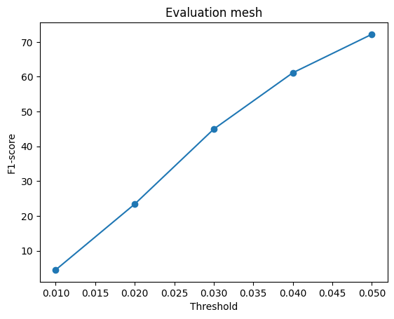
columns: input | prediction | GT mesh


Comparison of voxels vs points vs meshes
Ranking: point cloud (74.8) > mesh (72.2) > voxel grid (57.8).
Training iterations: voxel grid 10000, point cloud 4000, mesh 4000. Note the budgets are not equal (the voxel model was trained longest), so the ranking is, if anything, conservative for points and meshes.
| model | F1@0.01 | F1@0.02 | F1@0.03 | F1@0.04 | F1@0.05 |
|---|---|---|---|---|---|
| Voxel grid | 3.8 | 18.4 | 35.0 | 48.1 | 57.77 |
| Point cloud | 5.2 | 22.7 | 44.8 | 62.9 | 74.81 |
| Mesh | 4.5 | 23.4 | 45.0 | 61.1 | 72.20 |

- Point cloud: the point decoder places every output point freely and the Chamfer loss pulls each one onto the surface, so thin legs and slats are only limited by the number of points; there is no topology or resolution constraint.
- Mesh: the mesh is a deformed genus-0 ico-sphere: it cannot open the holes between legs, back slats or arm rests, so it stretches faces across them, and the Laplacian term additionally shrinks thin protrusions.
- Voxel grid: the 323 grid has a cell size of ~0.03, comparable to the 0.05 threshold, so thin parts are either missed (they occupy less than half a cell) or thickened; marching cubes on a thresholded grid adds a staircase surface and the extra alignment/recentring step in the evaluation also costs precision.
All three share the same encoder and data; the difference is the inductive bias of the output representation. F1 at a fixed distance threshold rewards getting many surface samples close to the GT, which favours the representation with the fewest structural constraints on where samples can go.
Observation. Part of the voxel gap is the representation itself, not the network: for the curved-shell chair below, even the ground-truth 323 voxelisation (last column) breaks the thin shell into disconnected slats, and for the thin folding chair the voxel prediction survives the 0.5 threshold only as a few fragments. Thin parts below one cell are where voxels lose, and they are exactly where the point decoder has no such limit.


2.4 Hyper-parameter analysis: w_smooth
Setup. To compare settings at equal cost, all four runs start from the same mesh checkpoint (2000 iterations with w_smooth = 0.1) and are then trained for 2000 further iterations with w_smooth ∈ {0, 0.1, 1, 5}; everything else (data order aside) is identical. The loss is Chamfer + w_smooth · Laplacian.
| model | F1@0.01 | F1@0.02 | F1@0.03 | F1@0.04 | F1@0.05 |
|---|---|---|---|---|---|
| w_smooth = 0 | 5.0 | 24.2 | 46.0 | 62.5 | 73.91 |
| w_smooth = 0.1 | 4.5 | 23.4 | 45.0 | 61.1 | 72.20 |
| w_smooth = 1 | 4.6 | 23.4 | 44.3 | 59.8 | 70.56 |
| w_smooth = 5 | 3.2 | 17.0 | 33.8 | 47.7 | 58.42 |

Result. F1@0.05 — w_smooth = 0: 73.9 , w_smooth = 0.1: 72.2 , w_smooth = 1: 70.6 , w_smooth = 5: 58.4. Best: w_smooth = 0 (73.9); worst: w_smooth = 5 (58.4).
Interpretation. F1 decreases monotonically as w_smooth grows (73.9 → 72.2 → 70.6 → 58.4). The Laplacian term pulls every vertex toward the centroid of its neighbours, i.e. it penalises curvature. A chair is mostly thin, high-curvature structure (legs, stretchers, slat edges) attached to a few flat panels, and the template is a genus-0 sphere that cannot open holes. A strong smoothness prior therefore shrinks legs and rounds off corners, pulling surface samples away from the GT; this is exactly what F1 at a fixed distance threshold punishes, and the drop is dramatic at w_smooth = 5 (58.4). In the other direction, removing the term entirely gives the best F1 (73.9) but only 1.7 points above w_smooth = 0.1: with Chamfer alone nothing couples neighbouring vertices, so the surface is free to become irregular (uneven triangles, folds), and F1, which only measures distances of sampled points, does not see this. The training-loss panel is consistent: the total loss rises with w_smooth because the two terms compete.
What the renders show (same test chairs below). F1 does not tell the whole story. At w_smooth = 0.1 the predicted surfaces are crumpled and self-intersecting: Chamfer only asks that sampled points lie near the GT, so the decoder scatters vertices onto the right region and the triangles between them fold through each other, which F1 barely penalises. At w_smooth = 1 the spikes are visibly reduced for only a small F1 cost. At w_smooth = 5 the surface becomes a smooth, closed sheet that has collapsed the legs and gaps entirely (thin folding chairs turn into a single curved blade), which is where F1 finally drops sharply.
Choice. For the metric alone, the weakest regulariser wins; for a usable surface, w_smooth ≈ 1 is the better trade-off (noticeably fewer folds and spikes for 1.6 F1 points less than w_smooth = 0.1), and values ≥ 5 over-smooth. Note that the R2N2 loader draws a random input view per test sample, so the input images in the comparison below differ between runs; the averaged F1 is unaffected, but individual renders are not a strictly controlled comparison.
same test sample (300) under each setting — columns: input | prediction | GT mesh


2.5 Interpreting the model
Four complementary probes, applied to the trained models; samples are chosen automatically as the two worst and the best test chairs by F1@0.05.
(a) Where is the error? Precision / recall heat-maps
Columns: input | prediction coloured by distance to the nearest GT point (precision error) | GT coloured by distance to the nearest predicted point (recall error); blue = 0, red ≥ 0.1. F1 averages these two failure modes, so separating them shows which one dominates.
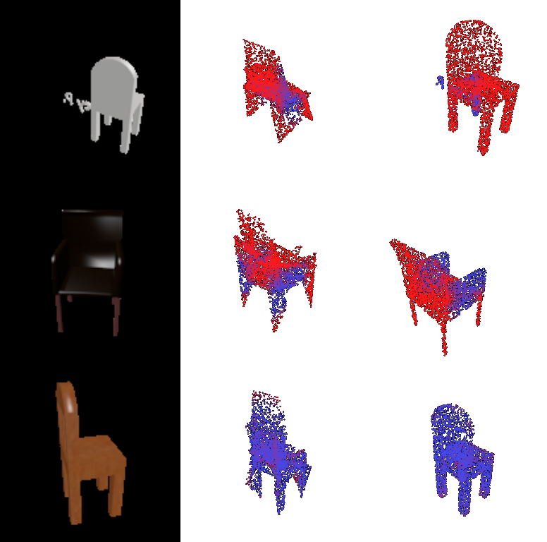
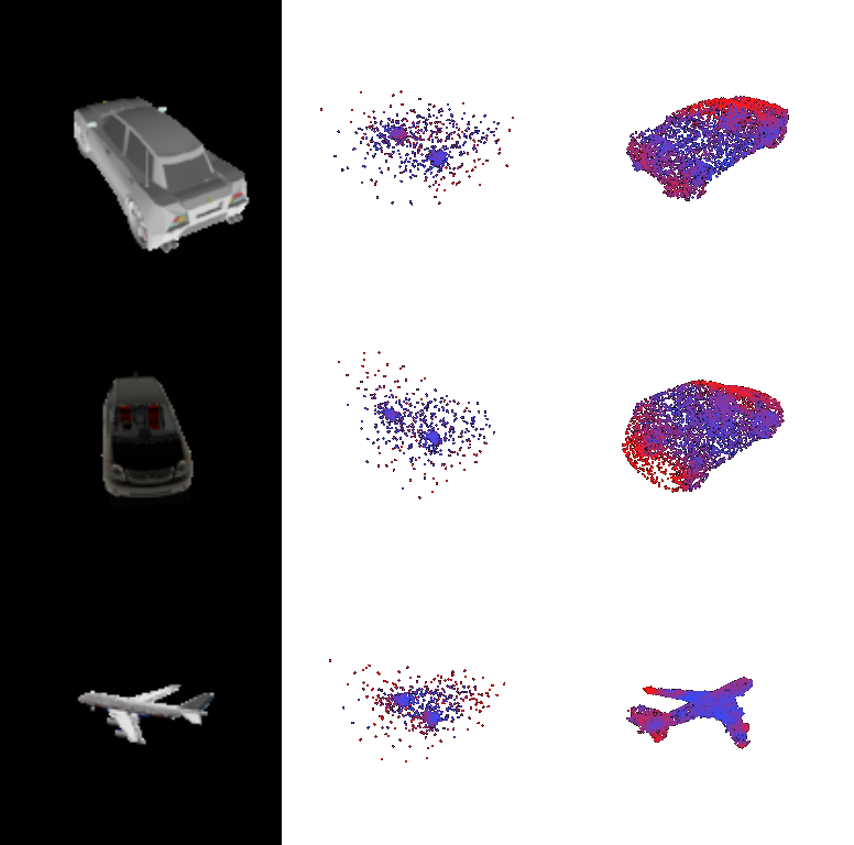
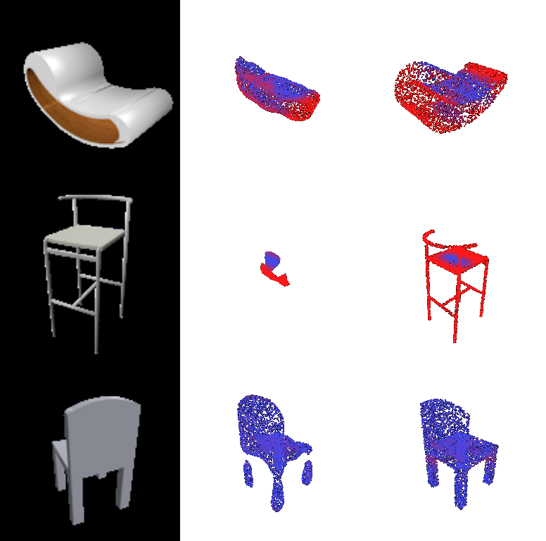
Findings. The two failure modes are not symmetric. For the worst chairs the GT is red almost everywhere on its thin parts — legs, stretchers, the top of the back — i.e. recall dominates: the network never puts geometry there. The clearest case is the voxel model on a bar stool with wire-thin legs, where the prediction is a small fragment around the seat and the whole frame is red. Precision errors (red on the prediction) appear in a different place for each representation: on the mesh they sit on the spiky fins that the crumpled surface throws out between parts, on the voxels at the ends of an unusual elongated lounge chair whose extent the model under-estimates. For the best chairs (solid, conventional four-legged shapes close to the class average) both maps are blue: the models do well exactly when the chair looks like the mean chair.
(b) Latent-space interpolation
The image codes zA, zB of two test chairs are linearly blended, (1−t)zA + t zB, and decoded. Leftmost/rightmost: input images. A smooth morph means the decoder has learned a continuous shape manifold rather than memorising discrete templates.

Findings. The morph is not linear in t. The first four steps decode to almost the same chair as the left input; the shape then changes abruptly over the last two steps into the spiky, splayed surface the model predicts for the right input. So the code space is continuous (no tearing or garbage in between), but the decoder output is flat over a large region around a typical chair and only moves once the code is close to an unusual one, consistent with a model that has learned a strong mean-chair prior with a few directions of variation.
(c) Sensitivity to the input viewpoint
The same chair is fed from 4 different R2N2 views (top row); bottom row shows each prediction rendered from one fixed camera. A view-invariant model would produce identical shapes.


| test chair | F1@0.05 per input view | mean | std |
|---|---|---|---|
| 653 | 14.8, 15.5, 15.0, 11.1 | 14.1 | 1.8 |
| 47 | 95.9, 96.8, 96.8, 96.7 | 96.5 | 0.4 |
Findings. The predictions are nearly identical across input views, even when the views differ strongly (front-left, back-right and a pure side view of the same chair). R2N2 ground truth is in the object's canonical frame, not the camera frame, so the network has to undo the viewpoint; it has learned to do so and outputs one canonical shape per chair. The flip side is that view-specific evidence, such as a leg visible in only one view, barely changes the output, which again points to a strong shape prior rather than detailed per-view reasoning.
(d) Voxel confidence
Every voxel with p > 0.05 drawn as a point coloured by its predicted occupancy probability (blue = uncertain, red = confident). The marching-cubes surface used for evaluation only keeps p > 0.5, so this shows what the threshold throws away.

Hedged voxels (0.2 < p < 0.8) relative to occupied voxels: chair 3: 6.10×, chair 423: 1.54×.
Findings. On a conventional chair, confidence is concentrated in the interior of the seat and back (red core), while the outer shell and especially the legs are blue: the network is unsure exactly where thin parts end, and the legs survive the 0.5 iso-level only partially. On an unusual lounge chair the whole volume is blue: the model spreads low probability over a plausible region instead of committing, which the fixed 0.5 threshold turns into missing or truncated geometry. This is the same hedging mechanism that leaves the implicit network (Q3.1) with empty predictions.
3. Other architectures / datasets
3.1 Implicit network
Model. f(z, p) → occupancy logit for a query point p ∈ (−1,1)3, evaluated on the 323 grid of voxel centres. p is Fourier-encoded (6 frequencies); since [z, PE(p)]·W = Wzz + WpPE(p), the image code is projected once per shape and broadcast-added to the per-point features, then re-injected into each of 4 residual MLP blocks (Occupancy-Network-style conditioning). Trained with the same BCE as the voxel decoder.
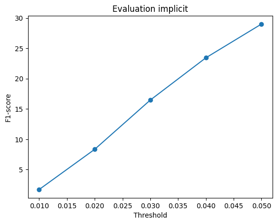
F1@0.05 = 28.99 (voxel decoder: 57.77), 10000 iterations, batch 16.
| model | F1@0.01 | F1@0.02 | F1@0.03 | F1@0.04 | F1@0.05 |
|---|---|---|---|---|---|
| Voxel decoder (3D deconv) | 3.8 | 18.4 | 35.0 | 48.1 | 57.77 |
| Implicit MLP | 1.7 | 8.3 | 16.5 | 23.4 | 28.99 |
columns: input | prediction | GT mesh | GT voxels
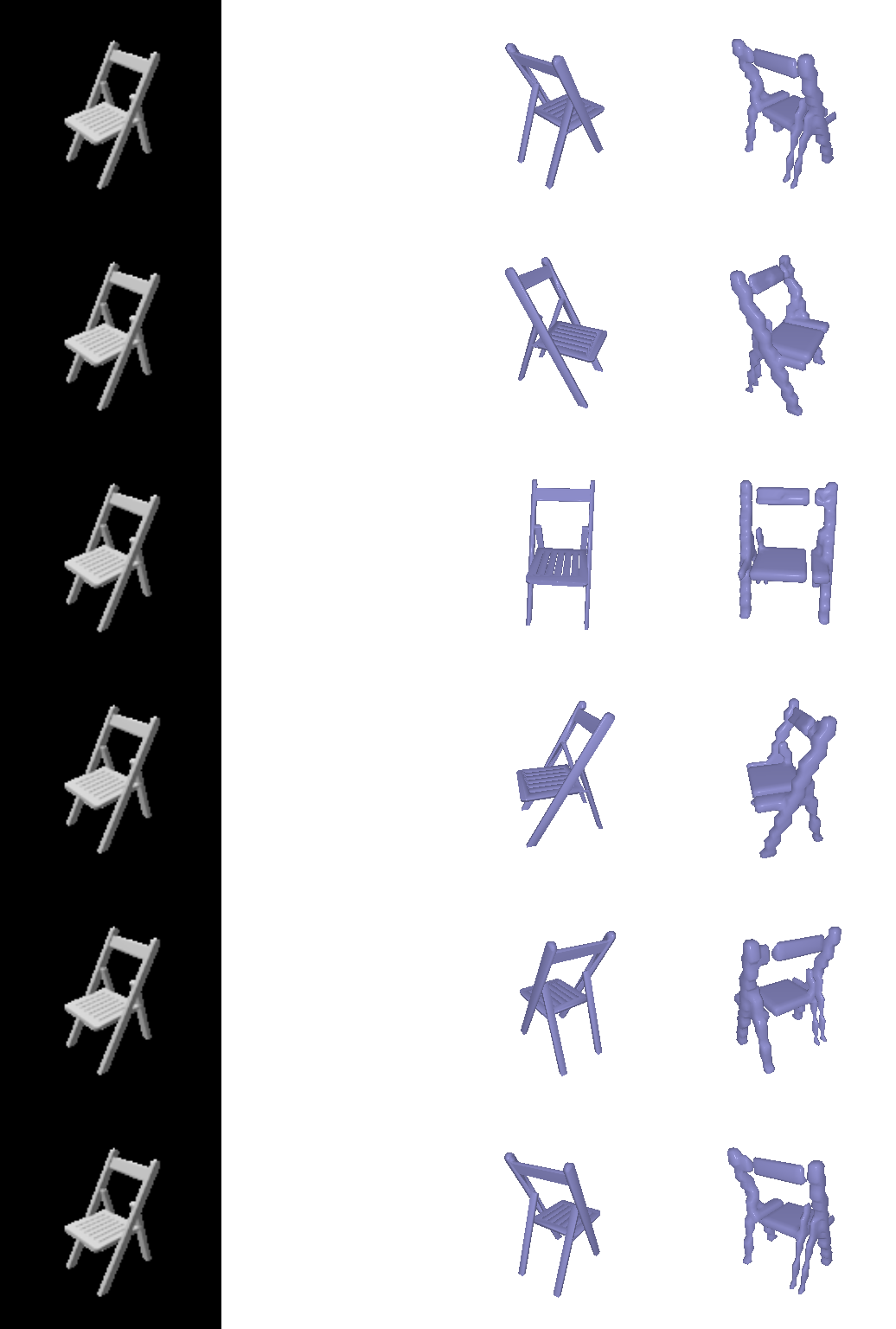
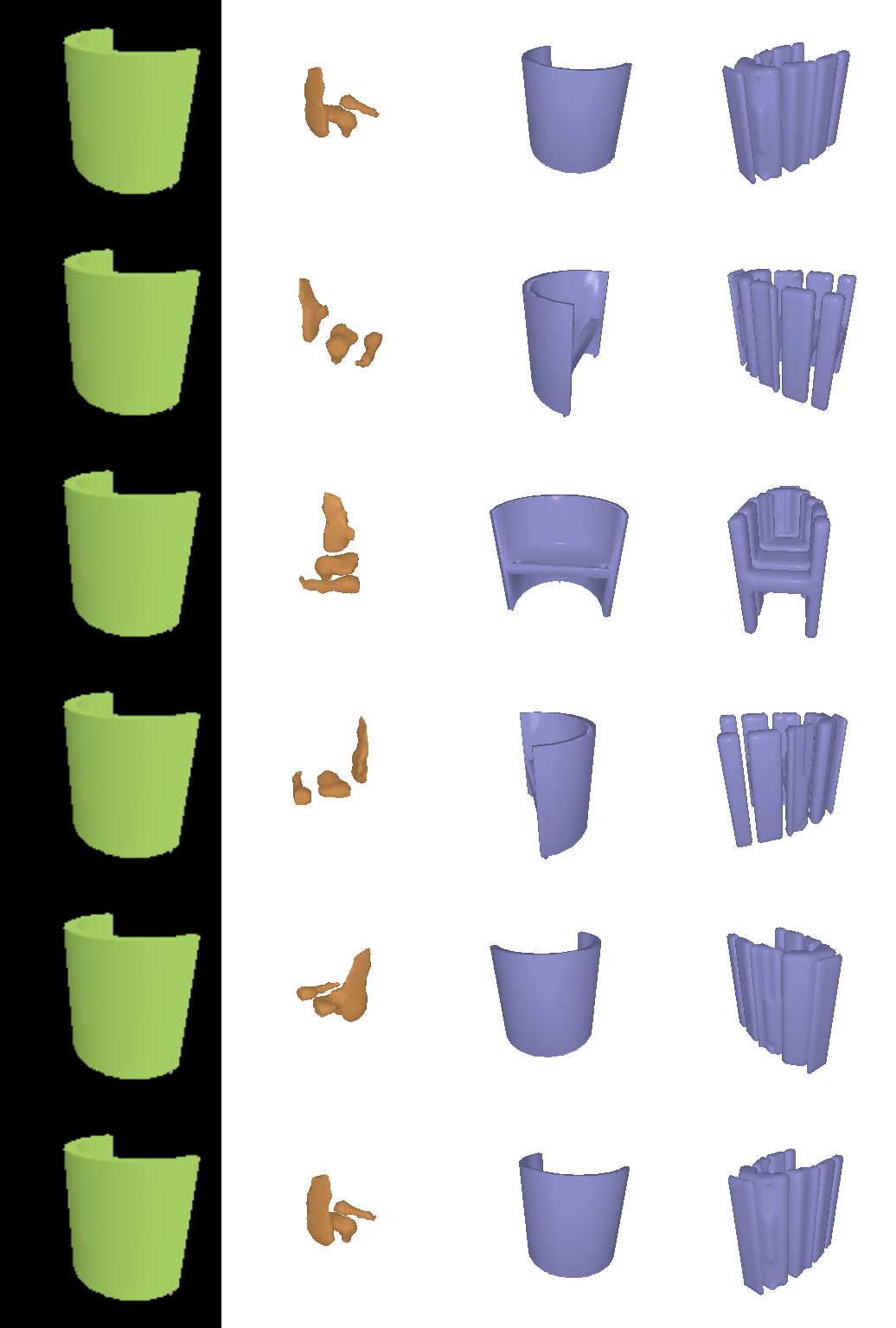
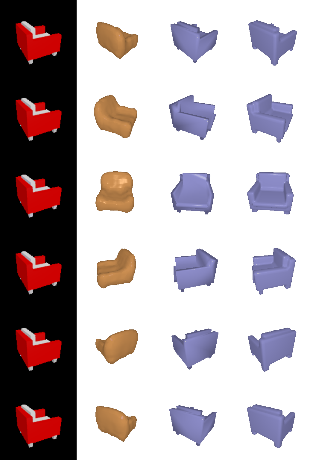
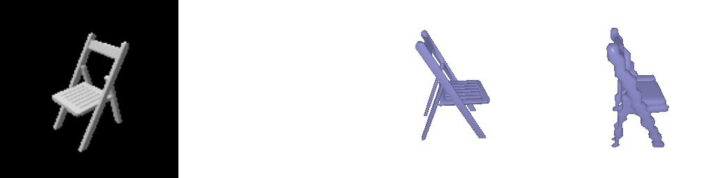
Analysis. The implicit MLP is clearly behind the 3D-deconvolution decoder (29.0 vs 57.8). 231 of 678 test chairs (34%) produce no voxel above p = 0.5 at all for the implicit model (an empty surface scores F1 = 0), versus 24 for the voxel decoder. The mechanism: the deconvolution decoder shares 3D kernels across the grid, so local structure (a leg is a vertical run of occupied cells) is learned once and reused everywhere; the MLP has no such spatial weight sharing and must learn the occupancy of every location from the global code alone, with ~0.5M parameters versus ~3.8M. Under the class imbalance (~10% occupied) an under-fitting occupancy network hedges, predicting p < 0.5 on thin parts and sometimes everywhere, and the fixed 0.5 iso-level of the evaluation then deletes them. Wider layers, more blocks, a per-point positive weight in the BCE, or local (pixel-aligned) image features as in PIFu would be the natural fixes; the advantage that remains is that the MLP is resolution-free and could be queried on a finer grid at test time. This is visible in the renders: on the thin folding chair (test sample 200) the implicit model outputs nothing above the threshold, and on the curved-shell chair (300) only a few disconnected blobs.

3.2 Parametric network
Model. AtlasNet-style: 4 charts, each an MLP φk(z, u), u ∈ [0,1]2 → R3. New u are sampled uniformly every forward pass, so the network learns a continuous surface map; trained with Chamfer like the point decoder.
F1@0.05 = 65.23 (point decoder: 74.81).
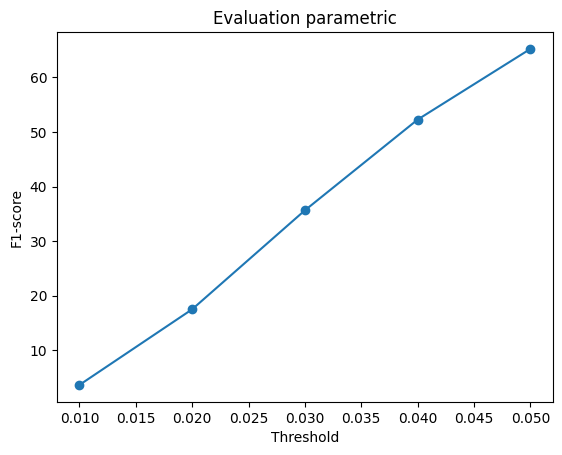
columns: input | points | charts as a surface (one colour per chart) | GT mesh
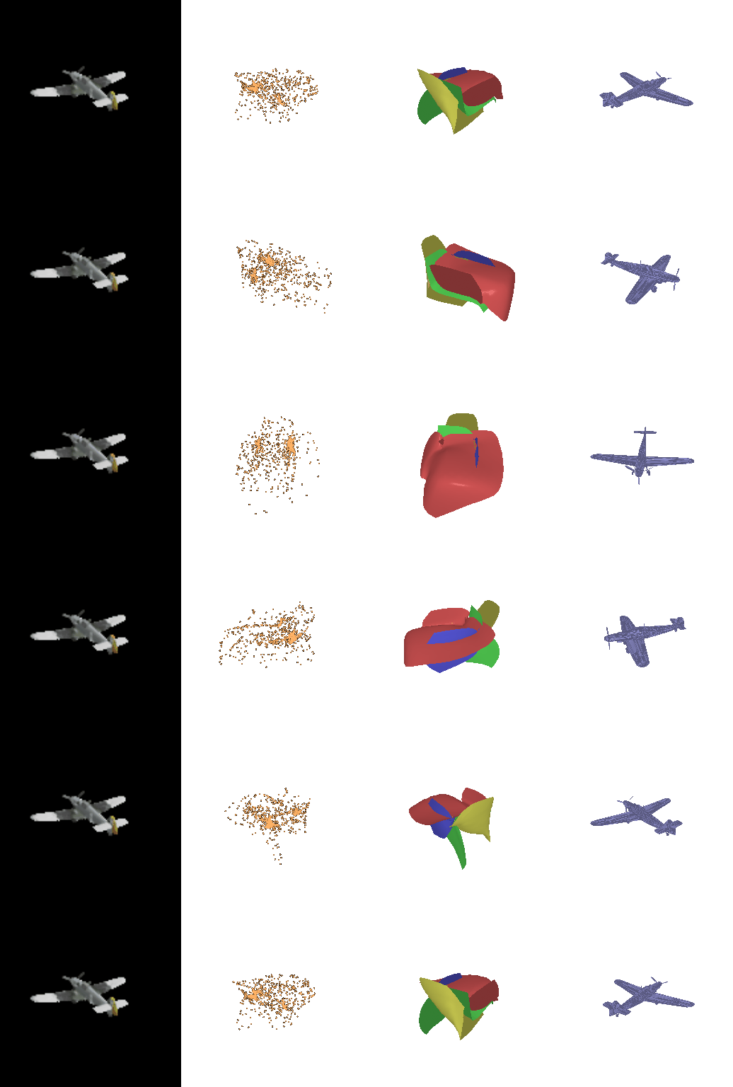
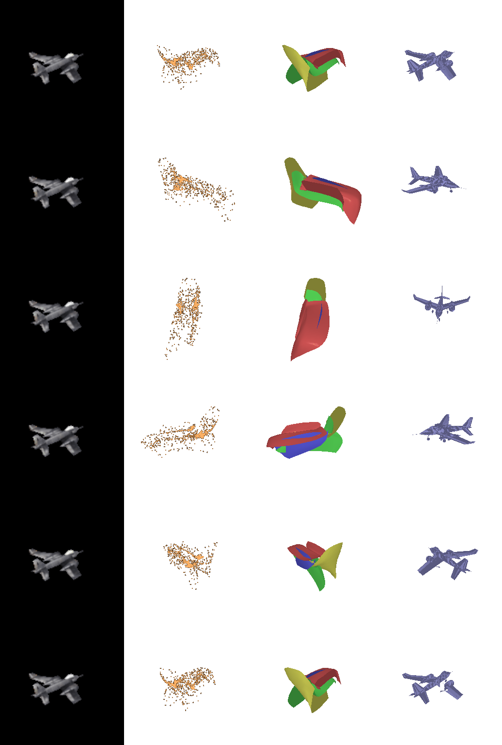
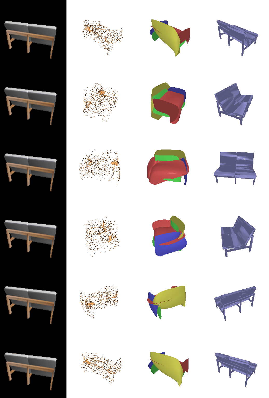
Analysis. The parametric decoder reaches 65.2 F1@0.05, below the free point decoder (74.8) and close to the deformed-sphere mesh (72.2), after 2000 iterations versus 4000 for the point model. Each chart is a continuous map of the unit square, so every output point lies on one of 4 smooth 2-manifold patches: this is a much stronger structural prior than independent points (a chart must stretch or fold to cover a thin leg, and neighbouring uv samples cannot jump between disconnected parts), but a weaker one than a single closed sphere, because the 4 patches need not be connected or watertight. F1 lands between the two accordingly. What the prior buys is a surface rather than a point set: the same network can be sampled at any density, and the coloured renders show how the charts split the chair into parts. The chart layout is consistent across chairs (one chart forms the back, one a large front/seat sheet, the others the sides and bottom), so the charts do specialise. However, after 2000 iterations the chart surfaces are very similar for an armchair and a thin folding chair: the decoder has learned the average chair layout, and most of the input-specific variation is still missing.