Assignment 4: Multi-View Transformers
16-825: Learning for 3D Vision · Name: Zixin Guo · Andrew ID: zixinguo
Part 1 prepares canonicalized multi-view data from ScanNet++ iPhone frames (a4data/geometry.py). Part 2 trains Mini-LVSM, a decoder-only transformer that renders a new view from source images and camera rays (models/lvsm/). Part 3 trains Mini-VGGT, which predicts cameras and depth from RGB alone (models/vggt/).
1. Multi-View Data Preprocessing
1.1–1.5 What each function does
resize_intrinsics: the crop is already applied, so only the resize is left. Withalign_corners=False, pixel centers map asx_out + 0.5 = s (x_in + 0.5), sofx, fyare multiplied bys = 224 / side, and the principal point becomess (c + 0.5) - 0.5. The-0.5offset matters: just multiplyingcbyswould shift every pixel by about a quarter pixel, and the final check would not reach 0.01 px.unproject_depth: builds the(u, v, 1)grid at integer pixel centers, multiplies byK⁻¹to get a ray withz = 1, scales it by the z-depth (not by the ray length, since the depth maps store optical-axis depth), then appliesX_world = R X_cam + t.canonicalize_cameras:T_ref←cam_i = T_world←cam_0⁻¹ · T_world←cam_i, computed in float64. Camera 0 becomes the identity. Points are unprojected in this frame,compute_scene_scalereturns the norm of the valid-point centroid, and translations, depth and points are all divided by it. Rotations are unchanged, and nothing is subtracted, so camera 0 stays at the origin.camera_rays: sameK⁻¹ (u, v, 1)directions, rotated byR(no translation for directions) and normalized to unit length. The origin of every ray of viewvis that camera’s centert_v.plucker_coordinates:m = o × d, output[d, m].
Visualizations
Points and cameras after unprojection (original world frame, meters). The red frustum is view 0, the black × is the valid-point centroid, and the dashed line connects camera 0 to the centroid.


Four of the eight sampled views of scene 036bce3393: resized RGB and the aligned z-depth (white = missing).
The same two scenes after canonicalization. Camera 0 sits at (0, 0, 0) and the centroid is exactly one unit away; the scene scale printed in the title is the centroid distance in meters before dividing.


check_data.py output
python scripts/check_data.py --config configs/scannetpp/iphone/data.json --split train --max-samples 4
| sequence | views | res | valid depth | max point reproj. (px) | max ray reproj. (px) | centroid distance |
|---|---|---|---|---|---|---|
e050c15a8d_frame_005750 |
8 | 224 | 0.952 | 1.2e-4 | 1.3e-4 | 1.000 |
5f99900f09_frame_003000 |
8 | 224 | 0.992 | 9.9e-5 | 8.9e-5 | 1.000 |
47b37eb6f9_frame_007760 |
8 | 224 | 0.975 | 1.0e-4 | 8.2e-5 | 1.000 |
4c5c60fa76_frame_010770 |
8 | 224 | 0.989 | 1.1e-4 | 8.6e-5 | 1.000 |
Batch shapes (B = 2, V = 8): rgb (2,8,3,224,224), depth/depth_valid (2,8,1,224,224), K (2,8,3,3), T_world_from_camera (2,8,4,4), points_world/ray_origins/ray_directions (2,8,3,224,224), plucker (2,8,6,224,224), scene_scale (2,). All reprojection errors are around 1e-4 px, far under the 0.01 px limit. The full JSON is in data/check_data_train.json.
Short explanations
Canonicalization. Every training sample is rewritten in the coordinate frame of its first camera and rescaled so the valid-point centroid is one unit from that camera. Without this, the model would see the same room at arbitrary positions, orientations and scales, depending on where the original ScanNet++ world origin happened to be. With it, “camera 0 is at the origin looking down +Z, and the stuff it sees is about one unit away” holds for every sample, so the network learns one consistent convention. It also makes the depth and translation targets of Part 3 well scaled (around 1) rather than in meters that vary by room. The centroid is used for the scale only; it is not subtracted, since camera 0 must stay at the origin.
World-space ray directions. A pixel (u, v) sees along K⁻¹ (u, v, 1) in camera coordinates. Rotating by R (the camera-to-world rotation) gives the same direction in the canonical world frame; the translation does not apply to directions. After normalization, each pixel stores a unit vector that depends on both the intrinsics and the camera orientation, so the model can tell where a pixel looks in the shared frame without being handed R or K explicitly.
Plücker moment. m = o × d is the cross product of the ray origin and its direction. It is the same for every point on the line ((o + λd) × d = o × d), so [d, m] identifies the line itself, not just a point on it. Together with d it encodes the camera position: two rays with the same direction from different cameras have different moments. |m| is the distance from the world origin to the line, so for camera 0 (origin at 0) all moments are zero, which is a clean way to mark the reference view.
2. Novel-View Synthesis with Mini-LVSM
2.0 Implementation notes
patchifyreshapes(…, C, H, W)to(L, C, gh, p, gw, p), permutes to(L, gh, gw, p, p, C)and flattens, so patches are row-major and each patch is stored in (row, col, channel) order.unpatchifyruns the same permutation backwards;unpatchify(patchify(x)) == xexactly.build_tokensadds the shared sincos positional embedding to source and target tokens, repeats theS·Nsource tokens for every target, appends that target’sNquery tokens and foldsTinto the batch. Each target is rendered in its own sequence, so targets never see each other (I checked that changing target 1’s rays leaves target 0’s output unchanged).forward:[2·rgb − 1, plücker]→patchify→source_proj; target rays →patchify→target_proj;input_norm, 8 transformer blocks, keep the lastNtokens,out_norm→rgb_head→ sigmoid →unpatchify.- Loss: plain
F.mse_lossover all target pixels. Training runs the forward under bf16 autocast and casts the prediction to float32 before the loss.
2.1 Overfitting
python -m models.lvsm.train --overfit 2000 --output-dir outputs/lvsm_overfit (one fixed batch of 4 samples, S = 2, T = 6; 9.4 min on an A40).
Final overfit PSNR: 30.94 dB (MSE 8.6e-4, SSIM 0.871) on the memorized batch. The loss went from 0.063 to below 1e-3; the mean PSNR over all 2000 training steps was 25.4 dB.

val_epoch000.png after 2000 overfit steps. Columns: source view 1, source view 2, ground truth target, prediction; one row per target view. The prediction matches the target, including the two targets (rows 2–3) that look at a very different part of the room than the sources, which can only be memorized, not inferred.
2.2 Training and evaluation
Settings (configs/lvsm.json, unchanged): patch 8 (784 tokens per view), width 384, 8 blocks, 6 heads of 64, QK-norm, 14.6M parameters. S = 2 sources and T = 6 targets out of V = 8 views sampled from a 32-frame window, batch 4 (24 target images per step). AdamW, lr 2e-4, weight decay 0.05, betas (0.9, 0.95), 200 warmup steps then cosine to 10 %, gradient clip 1.0, bf16 autocast. 100 epochs × 56 steps = 5600 steps; 2 h 16 min on one A40 (about 80 s per epoch, most of it data loading with 4 workers). Validation: 28 scenes, 8 views from the first 32 prepared frames, seed 825.

Training curves from log.jsonl. The validation PSNR was still going up at epoch 100 (16.13 dB, SSIM 0.560), so the model is limited by training time, not by overfitting. Train loss sits above val loss because the train numbers are averaged over an epoch while the weights are still moving, and because training windows come from anywhere in a scan while validation always uses the first 32 frames.
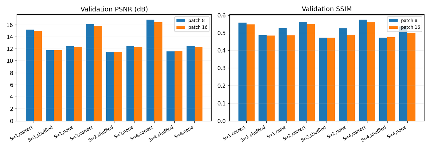
Validation metrics for every ablation (best.pt, 28 scenes; correct = true target rays, shuffled = rays of another target view, none = all-zero rays):
| sources S | conditioning | PSNR (dB) | SSIM | MSE | images |
|---|---|---|---|---|---|
| 1 | correct | 15.19 | 0.558 | 0.0352 | 196 |
| 1 | shuffled | 11.80 | 0.487 | 0.0729 | 196 |
| 1 | none | 12.47 | 0.527 | 0.0589 | 196 |
| 2 | correct | 16.13 | 0.560 | 0.0294 | 168 |
| 2 | shuffled | 11.49 | 0.472 | 0.0778 | 168 |
| 2 | none | 12.45 | 0.527 | 0.0591 | 168 |
| 4 | correct | 16.87 | 0.575 | 0.0247 | 112 |
| 4 | shuffled | 11.59 | 0.473 | 0.0783 | 112 |
| 4 | none | 12.45 | 0.537 | 0.0588 | 112 |
For reference, three trivial predictors on the same validation targets (S = 2): copy source view 0 → 10.95 dB / 0.354; average of the two sources → 12.00 dB / 0.372; a constant gray image → 12.04 dB / 0.538.


Training visualizations on the first validation batch (columns: 2 sources, GT, prediction). Left: epoch 0, the output is one flat color. Right: epoch 95, the layout (bright window, dark chair, table) is in the right place but everything is blurry at the 8 px patch level.
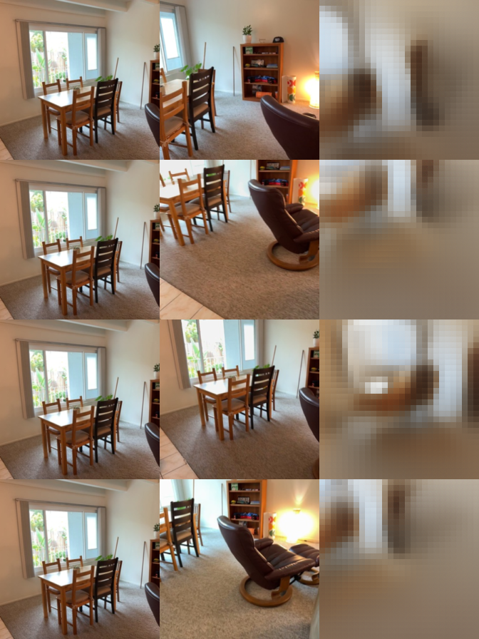
S = 1, correct rays
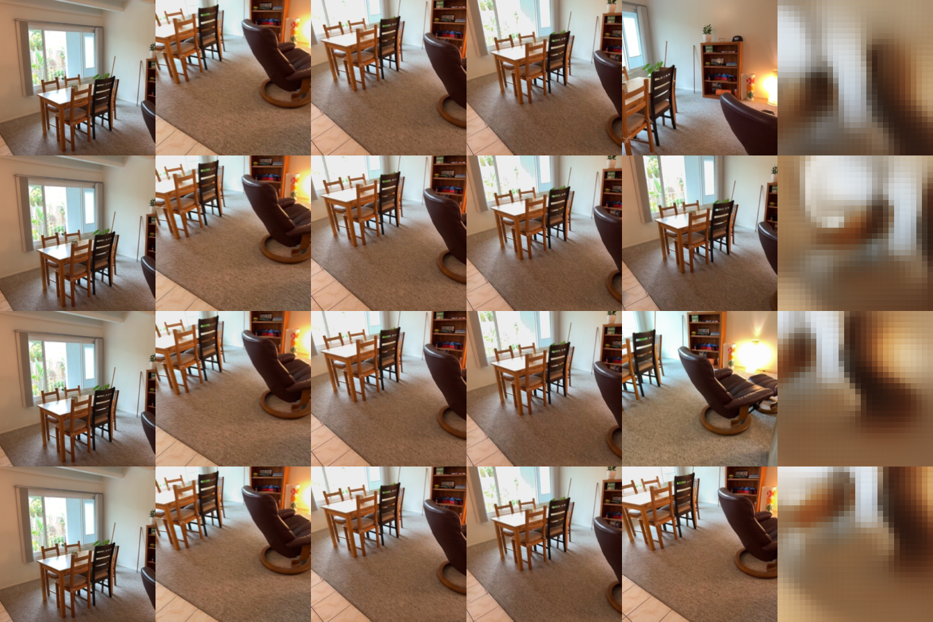
S = 4, correct rays
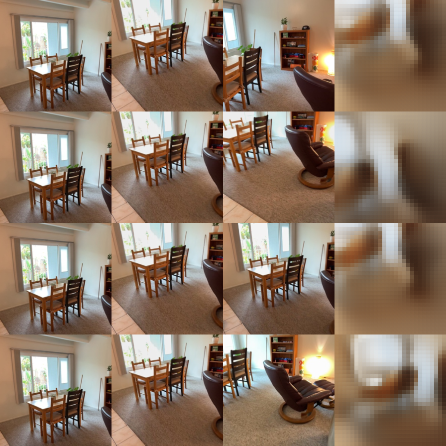
S = 2, shuffled rays
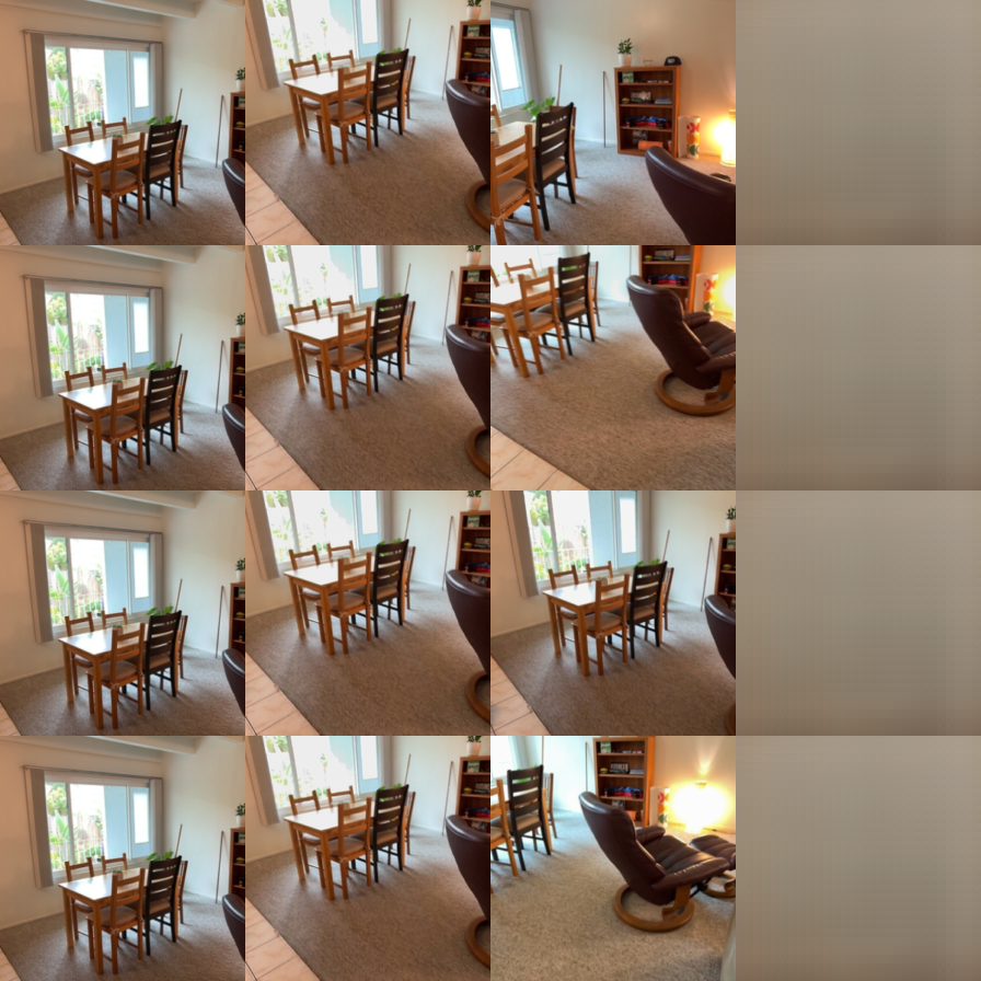
S = 2, zero rays
Number of source views. More sources help every time: 15.2 → 16.1 → 16.9 dB for 1 → 2 → 4 sources, even though the model was trained with exactly 2. Each extra source covers more of the target’s field of view and gives the attention more patches to copy color from. The gain from 2 → 4 (0.7 dB) is smaller than from 1 → 2 (0.9 dB), while the sequence gets longer (3920 vs 2352 tokens), so the cost grows faster than the quality.
Ray conditioning. The target rays are the only thing that tells the model which view to render, and the ablation shows it uses them. With zero rays the output is the same for every target and PSNR drops to 12.45 dB, almost exactly the “mean of the sources” and “flat gray” baselines (12.0 dB): the model falls back to an average image. Shuffled rays are even worse (11.5 dB), below the gray baseline, because the model confidently renders the wrong view, and a sharp wrong image costs more than a blur. This is what a pose-conditioned renderer should do, and it shows that the Plücker tokens carry the camera pose and not just a “this is a target” flag (the target_proj bias alone would give the none result).
What limits quality. 16–17 dB is 4–5 dB above copying a source, but the renders are clearly blurry. The main reason is training time: 5600 steps with 24 target images each is very little for a transformer trained from scratch (the real LVSM trains far longer with much larger batches), and the validation PSNR was still rising. The second reason is the data: 8 views inside a 32-frame iPhone window often look at different parts of the room (copying a source only gives 11 dB), so many target pixels are not visible in any source, and MSE pushes those toward a blurry mean.
2.3 Bonus: patch size (model capacity vs. cost)
Question. Mini-LVSM spends most of its compute on attention over (S+1)·N tokens. Doubling the patch size from 8 to 16 cuts N from 784 to 196 (4× fewer tokens, ~16× cheaper attention) but each token must now encode a 16×16×9 patch and the head must decode a 16×16×3 patch. How much quality does this cost, and how much time and memory does it save, at a fixed training budget?
Setup. configs/lvsm_p16.json is identical to the baseline except patch_size: 16 (same width, depth, optimizer, schedule, 100 epochs, batch 4, S = 2, same seed). The patch-16 run had to be split into four sub-1-hour Slurm jobs with --resume (the queue only let me use the interactive partition), which does not change the schedule. Speed and memory come from tools/bench_lvsm.py, which times forward + backward on one synthetic training batch (B = 4, S = 2, T = 6, 224 px, bf16) on the same A40, so data loading is excluded.
Results (validation, best.pt of each run):
| patch 8 (baseline) | patch 16 | |
|---|---|---|
| parameters | 14.6 M | 16.0 M (bigger in/out projections) |
| tokens per sequence (S = 2) | 2352 | 588 |
| train step, model only | 265 ms | 63 ms (4.2× faster) |
| inference, one batch | 84 ms | 19 ms |
| peak training memory | 8.9 GiB | 2.5 GiB |
| wall-clock per epoch (data-bound) | 80 s | 104 s* |
| PSNR / SSIM, S = 1 | 15.19 / 0.558 | 15.01 / 0.548 |
| PSNR / SSIM, S = 2 | 16.13 / 0.560 | 15.86 / 0.550 |
| PSNR / SSIM, S = 4 | 16.87 / 0.575 | 16.46 / 0.562 |
| PSNR, S = 2, shuffled / none rays | 11.49 / 12.45 | 11.52 / 12.33 |
Both runs are limited by the 4-worker data loader (JPEG/PNG decoding plus undistortion for 32 frames per step), not the GPU, so the wall-clock does not reflect the model cost; the patch-16 run was even slower per epoch because it shared its nodes with other interactive jobs.
Training curves of both runs. The two models track each other closely for the whole run; patch 8 pulls ahead by about 0.3 dB after epoch 40.

Same validation batch at epoch 95: patch 8 (left) vs. patch 16 (right). The 16 px blocks are plainly visible on the right; the coarse layout is the same.
Full ablation for both runs. The ray-conditioning pattern (correct ≫ none > shuffled) is identical for both patch sizes.
Conclusions.
- Patch 16 costs only 0.2–0.4 dB PSNR and about 0.01 SSIM at every source count, while the model itself is 4× faster to train, 4.4× faster at inference and uses 3.5× less memory. With 4× fewer tokens the attention part could be up to 16× cheaper; the measured 4× means the linear layers and the per-token head now take most of the time.
- The small quality gap says that, with this much training, the baseline is not held back by its 8 px grid. Both models give blurry, patch-level renders (see the pictures), and the blur comes from too little training and from target pixels that no source sees (section 2.2), not from the patch size. A finer grid only pays off once the model is good enough to draw detail.
- Patch 16 is the better deal when compute is limited: for the same GPU time it could train 4× more steps or use a 4× larger batch, and since the patch-8 validation PSNR was still rising at the end, that extra training would very likely win back more than the 0.3 dB.
- Limitations: one seed per setting, and the differences (0.2–0.4 dB) are about the size of the epoch-to-epoch noise in the curves, so the ranking is likely but not certain. The wall-clock comparison is distorted by the data loader; to actually benefit from the faster model, the loader needs more workers or pre-decoded frames. I also did not try a size in between (224 is not divisible by 12, so patch 14 or 28 would be the next choices) or widen the patch-16 model to match parameter counts.
3. Multi-View Geometry with Mini-VGGT
3.0 Implementation notes
aggregate: even blocks run frame attention on(B·V, N, D)with the per-view RoPE positions; odd blocks run global attention on(B, V·N, D)with the positions repeatedVtimes (no view-order embedding; camera 0 is marked by its own camera/register tokens). The output of the last frame block is saved before the last global block, and both are concatenated to2Dand passed throughself.norm.CameraHead.predict: the MLP outputs 9 numbers; translation and quaternion stay linear, the two FoV channels get a ReLU, all in float32.DepthHead.forward:denselinear →patches_to_image;refine(two 3×3 convs on[dense, rgb], applied onB·Vimages) is added as a residual; confidence uses its own linear +patches_to_image. Outputsexp(depth)and1 + exp(conf).- Losses.
camera_loss: mean L1 on translation (per-element clamp at 100) + mean L1 on the XYZW quaternion + 0.5 × mean L1 on FoV, compared directly againstpose_encoding(GT).depth_gradient_loss: at strides 1/2/4/8, absolute differences of the masked residual between neighbors (clamped at 100), summed over edges where both pixels are valid and divided by the number of valid pixels, then averaged over the four scales.depth_loss:trimmed_mean(|d − d*|)+trimmed_mean(c·|d − d*| − 0.2·log c)+ gradient term, using only finite, positive, GT-valid pixels.
3.1 Overfitting
python -m models.vggt.train --config configs/vggt.json --overfit --output outputs/vggt_overfit: one training clip (036bce3393, 8 views), 40 epochs × 25 steps, lr 1e-3, 5 min on an A40.

Total, camera and depth loss while overfitting one clip. The total goes negative because the confidence term c·err − 0.2·log c is negative once the error is small and the confidence is large.
After 40 epochs on the fixed clip: camera loss 0.0026, depth loss −0.188, depth AbsRel 0.036, δ1 0.957, mean rotation error 0.17°, mean translation-direction error 0.35°, joint pose AUC@5° 0.986.

GT (left) vs. cameras + depth predicted from RGB only (right) for the overfit clip, in canonical coordinates. The two clouds are visually identical; all eight frustums land on the GT ones.

RGB, GT depth and predicted depth for four of the eight views of the overfit clip (white = no GT depth, predictions are masked the same way).
3.2 Training and evaluation
Settings (configs/vggt.json defaults): frozen DINOv2 ViT-B/14, 8 frame/global pairs (16 blocks) of width 384 with 6 heads, camera head with 4 cross-view blocks, depth head with RGB refinement; 8 views from a 32-frame window, 224 px, batch 16, 16 data workers. AdamW lr 6e-4, weight decay 0.01, 10 warmup epochs then cosine to 5 %, gradient clip 1.0, bf16 autocast, loss = 5 × camera + 1 × depth. 1000 epochs × 14 steps = 14 000 steps; 8.7 h on one A40 (about 31 s per epoch). best.pt is epoch 874 (lowest validation loss).

Total, camera and depth loss (train and validation) over 1000 epochs. Both losses were still slowly decreasing at the end. The validation curve is below the training curve (train is averaged while the weights move, and random training windows are harder than the fixed first-32-frame validation windows), so there is no overfitting.
Metrics (best.pt, 8 views from the first 32 prepared frames, 224 px, seed 825; 28 scenes = 784 camera pairs per split, no degenerate pairs):
| split | Depth AbsRel ↓ | Depth δ1 ↑ | Rot. AUC @5/15/30° ↑ | Trans. AUC @5/15/30° ↑ | Joint AUC @5/15/30° ↑ | mean rot. err | mean trans. err |
|---|---|---|---|---|---|---|---|
| val | 0.139 | 0.848 | 0.197 / 0.522 / 0.706 | 0.031 / 0.104 / 0.218 | 0.011 / 0.077 / 0.191 | 11.8° | 39.3° |
| test | 0.151 | 0.802 | 0.208 / 0.541 / 0.739 | 0.011 / 0.054 / 0.168 | 0.002 / 0.029 / 0.146 | 9.1° | 40.8° |
(Untrained model at epoch 0 on val: AbsRel 0.726, δ1 0.247, rotation AUC@30 0.286, translation AUC@30 0.0.)
GT vs. prediction on four validation scenes. Left: GT cameras and depth-unprojected points; right: the same views reconstructed from the predicted cameras and predicted depth. Below each: RGB, GT depth and predicted depth for four of the eight views.


09c1414f1b: living room. Layout, floor and far wall are right; the chairs become blocks and the predicted frustums are slightly rotated.


21d970d8de.

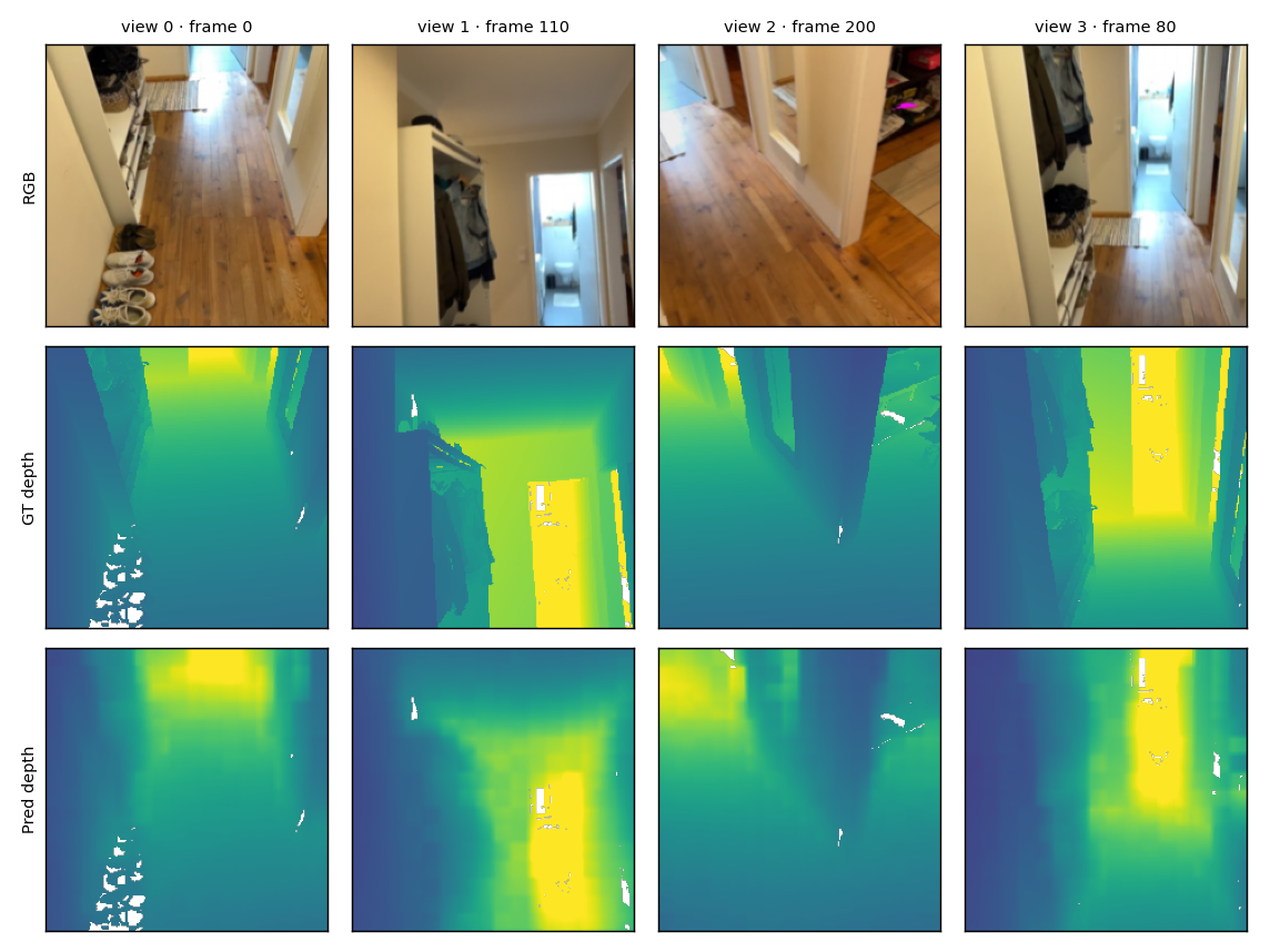
280b83fcf3: a narrow view with a lot of missing GT depth; the predicted cloud is wider and shallower than the GT.


2b1dc6d6a5: office. The chair and desk come out as coarse blobs, and the wall on the right is predicted closer than it is.
Errors on held-out scenes.
- Depth is coarse. The depth head decodes one linear layer per 14×14 DINO patch, and only a tiny two-layer conv works at full resolution, so predictions are blocky at patch borders (see every chair leg and table edge above). AbsRel 0.14–0.15 and δ1 0.80–0.85 mean the depth is within about 15 % for most pixels, but thin objects and edges are smeared over the whole patch. The depth order (floor near, wall far) is almost always right; the overall scale is what drifts, since the scale is set by the centroid of all views and the model has to guess it from appearance.
- Rotation is decent, translation is weak. About 70 % of the view pairs are within 30° of rotation and half are within 15°, but the translation direction is within 30° for only 22 % (val) / 17 % (test) of pairs. In a 32-frame iPhone clip the camera moves only a few tens of centimeters, so after normalization the translation vectors are short and their direction is hard to pin down, both for the model and for the metric (a small error in position becomes a large error in angle). This is also why the joint AUC, which takes the worse of the two, mostly follows the translation AUC.
- Test vs. val. Depth is a bit worse on test (0.151 vs 0.139 AbsRel), translation AUC is lower, rotation AUC is a bit higher; with 28 scenes per split this is normal scene-to-scene variation. The train/val loss gap is small, so the model is limited by its size and training time, not by memorizing.
- Failure modes. Missing GT around windows and shiny surfaces (white areas) is left out of the loss, so the model is never trained there and fills those areas with smooth guesses. Views that share very little with camera 0 (e.g. view 2 of
09c1414f1b, which looks at the floor) get the worst poses, since the global attention has few matching patches to anchor them.
3.3 Bonus: number of input views at test time
Question. The model was trained with exactly 8 views. How do accuracy, runtime and memory change when the same weights are given 2, 4, 8, 12 or 16 views of a scene?
Setup. tools/vggt_view_sweep.py evaluates best.pt on the 28 validation scenes with V ∈ {2, 4, 8, 12, 16} views drawn from the first 32 prepared frames (frame 0 is always the reference; smaller sets are prefixes of the same random permutation, so the 2-view set is a subset of the 8-view set). Batch size 4 on one A40; time is wall-clock for the whole split, memory is peak allocated.
| views | Depth AbsRel ↓ | Depth δ1 ↑ | Rot. AUC @15/30° | Trans. AUC @15/30° | Joint AUC @15/30° | pairs | s / scene | peak GPU mem |
|---|---|---|---|---|---|---|---|---|
| 2 | 0.110 | 0.875 | 0.579 / 0.719 | 0.174 / 0.306 | 0.143 / 0.281 | 28 | 0.10 | 0.76 GiB |
| 4 | 0.123 | 0.872 | 0.513 / 0.673 | 0.120 / 0.231 | 0.072 / 0.180 | 168 | 0.09 | 0.84 GiB |
| 8 (trained) | 0.139 | 0.848 | 0.522 / 0.706 | 0.104 / 0.218 | 0.077 / 0.191 | 784 | 0.15 | 1.00 GiB |
| 12 | 0.147 | 0.815 | 0.501 / 0.691 | 0.088 / 0.197 | 0.061 / 0.170 | 1848 | 0.40 | 1.16 GiB |
| 16 | 0.155 | 0.813 | 0.481 / 0.675 | 0.080 / 0.183 | 0.056 / 0.158 | 3360 | 0.79 | 1.32 GiB |
Results and explanation.
- Cost. Frame attention is linear in
V, global attention is quadratic: time per scene grows from 0.10 s (2 views) to 0.79 s (16 views), about 5× from 8 to 16 views for 2× the images. Memory grows roughly linearly here (0.76 → 1.32 GiB) because the batch is small and activations, not attention matrices, dominate; at training batch sizes the quadratic term would matter more. - More views do not help this model. Every metric gets worse from 8 to 12 to 16 views. The model never saw more than 8 views in training, so with 16 views each global-attention softmax is spread over twice as many tokens (4176 instead of 2088), which dilutes the attention to the matching patches. There is also no view-order embedding, so the extra views are only distinguished by content.
- Fewer views look better, with a caveat. 2 views give the best numbers, but the comparison is not entirely fair: with 2 views there are only 28 pairs, all involving the reference frame (whose pose is trivially the identity, and whose depth benefits from the camera-0 tokens), and the scene scale is recomputed from just two views, so the per-pixel targets differ slightly. The 2 → 4 → 8 trend on depth (0.110 → 0.123 → 0.139) is still informative: adding views adds frames that are farther from the reference and harder to place, and the model’s per-view depth gets slightly worse as the global context grows. A model trained with a random number of views (as the real VGGT is) would be the right fix; here that would mean another 9-hour run, so I report the test-time behavior only.
- Takeaway. For this Mini-VGGT, running at the training view count (or fewer) is the right choice; feeding more views costs 5× the time for worse accuracy. Generalizing to more views than seen in training requires training with varied view counts.