Assignment 3: Volume Rendering, NeRF, and 3D Gaussian Splatting
16-825: Learning for 3D Vision · Name: Zixin Guo · Andrew ID: zixinguo
Part A (nerf/) builds a differentiable volume renderer from scratch and uses it to fit a box, a NeRF and a VolSDF surface. Part B (GS/) builds a 3D Gaussian rasterizer in plain PyTorch, renders a pre-trained chair with it, and trains Gaussians on a toy truck and on the harder materials scene.
A. Neural Volume Rendering
1.3 Ray sampling
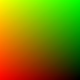
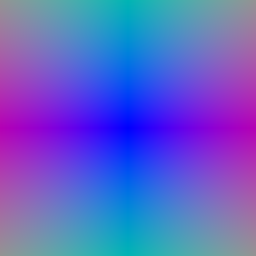
get_pixels_from_image makes one (x, y) pair per pixel with x = 2 i / (W - 1) - 1 and y = 2 j / (H - 1) - 1, so the corners land exactly on ±1 (this matches grid_sample(align_corners=True), which is what sample_images_at_xy uses later). get_rays_from_pixels appends z = 1 to each pixel, calls camera.unproject_points to get a world-space point on the image plane, and sets the ray origin to camera.get_camera_center(). The direction is the difference, normalized to unit length, so that later the ray lengths are real distances.
1.4 Point sampling
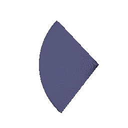
StratifiedRaysampler takes n_pts_per_ray evenly spaced depths between min_depth and max_depth with torch.linspace, and places a point at origin + t * direction for each. The depths are stored in sample_lengths so the renderer can turn them into segment lengths and into a depth map.
1.5 Volume rendering
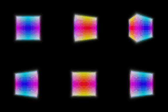
_compute_weights turns density into alpha = 1 - exp(-sigma * delta), builds the transmittance as a cumulative product of (1 - alpha) shifted by one (so the first segment has T = 1), and returns T * alpha. _aggregate is a weighted sum over the samples. forward uses it twice: once with the colours and once with the sample depths, which gives the depth map for free.
2. Optimizing a basic implicit volume
2.1–2.2 Random ray sampling and loss
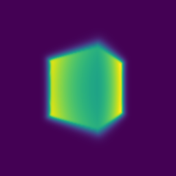
get_random_pixels_from_image shuffles the full pixel grid with torch.randperm and keeps the first n_pixels. The loss is the mean squared error between the rendered colours and rgb_gt. After 1000 epochs the box parameters are:
- center:
(0.25, 0.25, 0.00) - side lengths:
(2.01, 1.50, 1.50)
(Raw values: center (0.2502, 0.2506, -0.0004), sides (2.0051, 1.5036, 1.5034).) The box started at the origin with side 1.5 and the loss went from 0.044 to about 1e-6, so the four views pin it down well: the ground-truth box is at (0.25, 0.25, 0) with sides (2, 1.5, 1.5) and the fit is within a hundredth on every number.
2.3 Visualization
3. Optimizing a Neural Radiance Field
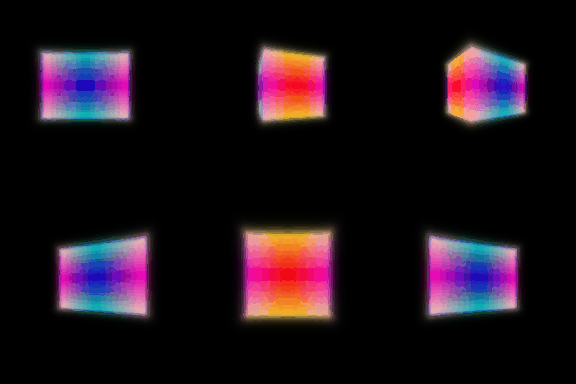
NeuralRadianceField is a plain MLP. The 3D point goes through the provided HarmonicEmbedding (6 frequencies, 39 numbers), then through MLPWithInputSkips with 6 layers of width 128 and the input appended again at layer 3, as in the NeRF paper. One linear layer plus ReLU gives the density, and a two-layer head (128 → 64 → 3) plus Sigmoid gives the colour. Training uses the same MSE loss as part 2, 1024 rays per step, 128 points per ray, 250 epochs on 128×128 images.
One thing I encountered: with the default seed the trunk output has a standard deviation of only 0.06 after six layers, and the random bias of the density layer came out at -0.11, so every density was negative before the ReLU, the output was black everywhere and the gradient was exactly zero. The loss sat at 0.08 for 250 epochs. Starting the density bias at +0.1 (one init.constant_ call) fixes it; after that the loss goes to about 0.003.

4. NeRF extras
4.1 View dependence
I added a use_view_dirs switch to NeuralRadianceField. When it is on, the ray direction is encoded with HarmonicEmbedding(3, 2) and concatenated to the 128-d feature right before the colour head; the density head does not see the direction. This is the split NeRF uses: geometry depends only on position, appearance may also depend on where you look from. I trained the materials scene twice with configs/nerf_materials.yaml, once without and once with the switch.


The scene is nine spheres with different materials, so view dependence matters here. With the direction as input, the training MSE over the last ten epochs drops from 0.0048 to 0.0039 (about 20 % lower), and in the gif the shiny spheres get a bright highlight that moves with the camera, while the position-only model paints each sphere a flat average colour; it cannot do anything else, because the same point must have the same colour from every direction.
An observed trade-offs. View dependence lets the model explain highlights, reflections and other effects that change with the camera, so it fits the training images better. The cost is that the extra freedom can also be used to memorize the training views: the network can give a point a different colour for every training direction instead of finding the right geometry, and then novel views, whose directions it never saw, look wrong or flicker. Two things keep this in check and both are in my implementation: the direction only enters after the density is computed, so geometry stays view-independent and must agree across all views; and the direction is encoded with few frequencies (2 here vs. 6 for position) and goes through a small head (one 64-wide layer), so the colour can only vary smoothly with direction. Dropping the direction into the trunk, or giving it a high-frequency encoding, would improve the training loss further but generalize worse. With only 100 training views of a 128×128 scene this is the right side of the trade-off to be on.
4.3 VolSDF
Distance MLP. NeuralSurface uses the same backbone as the NeRF (harmonic embedding, 6 layers of width 128) but the last layer is a plain linear layer with no activation, because a signed distance can be negative; its output is added to the distance to a unit sphere (see “Settings” below for why). A second small MLP (2 layers, width 128) takes the 128-d feature and outputs the colour with a Sigmoid. get_distance_color runs the backbone once and both heads, which is cheaper than two separate calls.
Eikonal loss. eikonal_loss is mean((||grad|| - 1)^2) over the gradients at random points in the bounds. It pushes the network to be a real distance field: moving one unit in space should change the predicted distance by one unit.
SDF to density. sdf_to_density follows section 3.1 of VolSDF: sigma(x) = alpha * Psi_beta(-d(x)), where Psi_beta is the CDF of a zero-mean Laplace distribution with scale beta. Written out, for s = -d:
sigma = alpha * 0.5 * exp(s / beta)          if s <= 0   (outside the surface)
sigma = alpha * (1 - 0.5 * exp(-s / beta))   if s > 0    (inside the surface)
What alpha and beta do. alpha is the density deep inside the object; the curve goes from 0 far outside to alpha far inside, and it is exactly alpha / 2 on the surface. beta is how wide the transition is. A small beta makes the density jump from 0 to alpha within a thin shell around the zero level set; a large beta smears that jump over a thick band.
- How does high
betabias the learned SDF? What about lowbeta? With a highbetathe renderer sees a soft, blurry object, so the SDF only needs to be roughly right near the surface: the loss barely changes if the zero level set moves a bit, and the result is a smooth, slightly inflated surface with washed-out detail. With a lowbetathe density is almost a step function, so the SDF is forced to put its zero crossing exactly where the colour changes, which gives sharp geometry but also lets small errors in the SDF show up as holes or floaters. - Is an SDF easier to train with low or high
beta? Highbeta. The density, and therefore the rendered colour, changes smoothly with the SDF everywhere, so gradients reach the network from a wide band of samples and from the start of training, when the surface is still in the wrong place. With a lowbetaalmost every sample has density 0 oralpha, the gradient with respect to the distance is close to zero except in a very thin shell, and if that shell does not line up with the true surface the network gets almost no signal. - Which gives a more accurate surface? Low
beta, once training is stable. The rendered colour comes from a thin shell around the zero level set, so the zero level set itself has to match the images. With highbetacolour is integrated over a thick band, and many different SDFs explain the images equally well, so the extracted surface (zero crossing) is blurry and tends to be too fat.
Settings. I used the defaults in configs/volsdf_surface.yaml: alpha = 10, beta = 0.05, eikonal weight 0.02, 128 samples per ray between depths 2 and 6, lr 5e-4 decayed by 0.8 every 50 epochs. beta = 0.05 is small compared to the scene size (the bulldozer is about 2 units wide) so the surface is already sharp, but it is not so small that the first epochs get no gradient; alpha = 10 makes a 0.05-thick shell almost opaque (1 - exp(-10 * 0.05 * 128 / 4) is essentially 1) so colours do not bleed through the object. The eikonal weight 0.02 is enough to keep the distance field well behaved without fighting the photometric loss.
The one thing I had to add is a geometric initialization. My first run predicted the distance directly from the MLP: at init the SDF is about 0 everywhere, so the whole volume is grey fog with density alpha / 2. Later I found that the quickest way to lower the loss on the mostly black background is to push the SDF positive everywhere, and the network did exactly that. Once d >> beta the density is exp(-d / beta), essentially zero with essentially zero gradient, so the object never came back; the render stayed black and marching cubes reported an empty mesh for all 250 epochs. A possible fix is the usual one for SDF networks: the MLP now predicts a residual on top of a sphere, d(x) = MLP(x) + (||x|| - 1). Training starts from a solid unit ball in the middle of the scene (which is also where the bulldozer is) and carves it down, and the eikonal loss is already small at init because the sphere term has unit gradient. With that change the loss goes to about 0.008 (0.003 of it is the eikonal term) and the surface comes out close to the TA’s.


B. 3D Gaussian Splatting
5. 3D Gaussian rasterization
- 5.1 Projection.
compute_cov_3DisR S Sᵀ RᵀwithR = quaternion_to_matrix(quats)andS = diag(scales); for isotropic Gaussians the quaternion is always the identity, so it reduces tos² Iand I skip the matrix products.compute_cov_2Dis equation (5) of the paper,J W Σ Wᵀ Jᵀ, withJfrom the provided_compute_jacobianandWthe camera rotation.compute_means_2Discamera.transform_points_screen(means)[:, :2], which already gives pixel units. - 5.2 Evaluation.
evaluate_gaussian_2Dcomputes-½ (x - μ)ᵀ Σ⁻¹ (x - μ)for every pixel and every Gaussian with oneeinsum.python unit_test_gaussians.pyprints[4/4] Tests Passed. - 5.3 Filter and sort. Depth is the
zof the mean in view space (get_world_to_view_transform().transform_points).get_idxs_to_filter_and_sortargsorts the depths and drops indices whose depth is not positive. - 5.4 Alphas and transmittance.
alpha = opacity * exp(power); transmittance is a cumulative product over the Gaussian axis of[S, 1 - α₁, 1 - α₂, …]with the last entry dropped, so GaussianiseesS ∏_{j<i}(1 - α_j)andScarries the value over from the previous mini-batch. - 5.5 Splatting. With
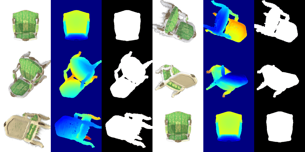
w = α T, the image isΣ w c, the depth isΣ w zand the mask isΣ w.render.pyjust callsscene.render(camera, per_splat=args.gaussians_per_splat, img_size=img_size, bg_colour=(1, 1, 1)).
6. Training 3D Gaussian representations
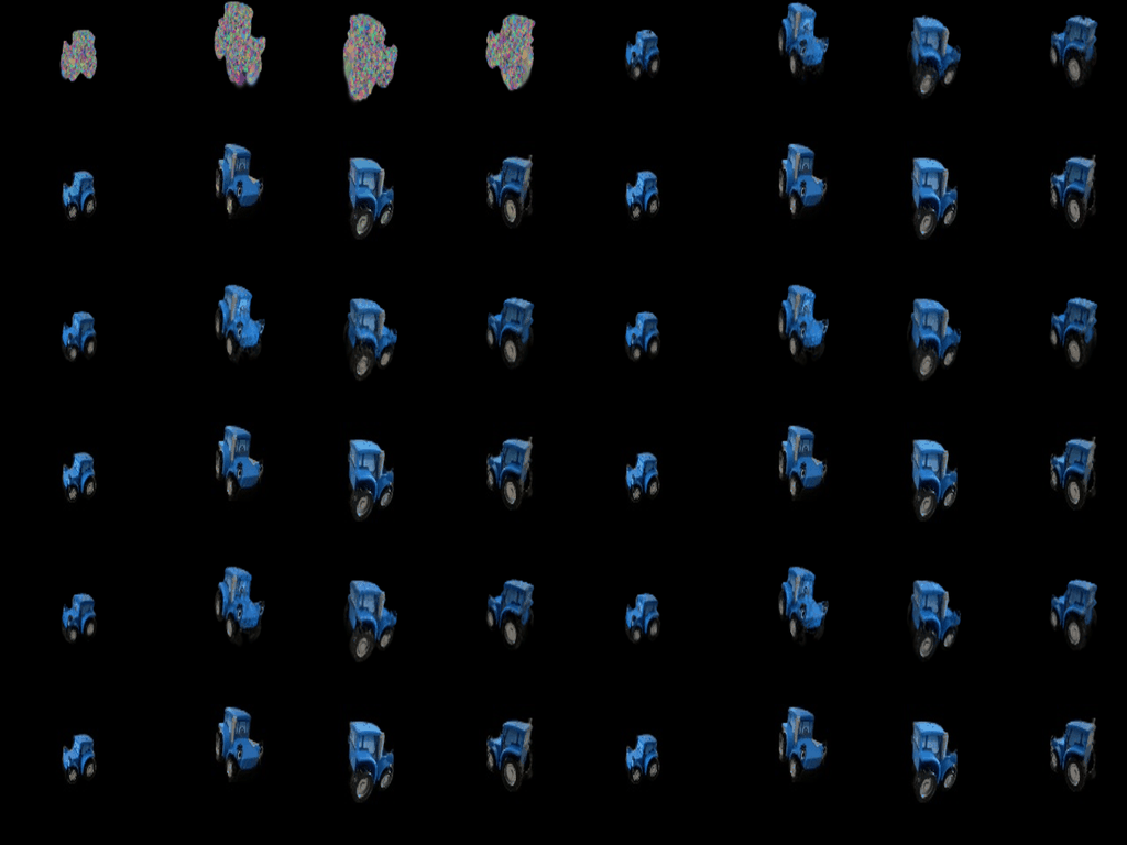
make_trainable sets requires_grad on the means, pre-activation scales, colours and pre-activation opacities (and on the quaternions only in the anisotropic case). The optimizer is Adam with one parameter group per attribute and the loss is L1 between the rendered image and the ground truth, with a black background.
- Learning rates: means
1e-3, scales (log-space)5e-3, colours1e-2, opacities (logit-space)5e-2. - Iterations: 1000 (the default), one training view per iteration.
- Held-out views: PSNR 29.88, SSIM 0.943 (mean over the 5 test views). The L1 loss went from 0.05 to about 0.006.
The means get the smallest rate because a Gaussian that moves too far in one step tears a hole where it was and leaves a blob where it lands, and the point-cloud initialization is already good. Opacities and colours are safe to move fast; they are bounded by the sigmoid and start from random colours anyway.

7.1 Rendering using spherical harmonics
colours_from_spherical_harmonics is a vectorized copy of the degree-3 real spherical harmonics evaluation from the reference implementation: the 48 coefficients are reshaped to (N, 16, 3), the 16 basis functions are evaluated from the direction (x, y, z), the result is shifted by 0.5 and clamped at 0. calculate_gaussian_directions normalizes means - camera.get_camera_center(). render.py has a --use_sh flag so both versions can be produced; the Gaussians keep their SH table only when the .ply provides one, so the training code in Q6/Q7.2 is not affected.
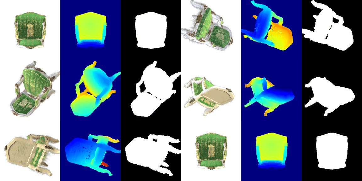
Three frames of the same spiral, DC colour on the left and full spherical harmonics on the right:


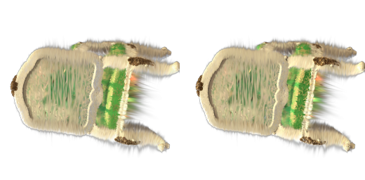
Overall the SH render looks less washed out. The DC coefficient is the mean of the colour over the sphere of directions, so every view gets the same average colour and the specular and shading changes between views are lost. The higher-order terms put that variation back.
7.2 Training on a harder scene
Baseline. train_harder_scene.py with the exact Q6 setup (isotropic Gaussians, the same learning rates, L1 loss, 1000 iterations) on materials with init_type="random": PSNR 18.66, SSIM 0.696. The L1 loss only gets down to about 0.05. In the progress gif the renders are a cluster of blurry blobs with roughly the right colours, bunched up near the middle of the image. The spheres near the edge of the scene are missing or very faint, because the random init puts every Gaussian in a small ball around the origin and the small learning rate on the means (0.001) is not enough to move them out to where those spheres are in 1000 steps.
Improved. Anisotropic Gaussians, means initialized in a wider ball (std 0.5 instead of 0.2), loss 0.8 * L1 + 0.2 * (1 - SSIM), means learning rate 0.005 decayed exponentially to 0.0005, 2000 iterations: PSNR 23.36, SSIM 0.864. Every sphere in the scene is now rendered in the right place with the right colour, and the loss goes down to about 0.03–0.04 (L1+SSIM) instead of flattening at 0.05 (L1).
| PSNR | SSIM | |
|---|---|---|
| Baseline (Q6 setup, random init) | 18.66 | 0.696 |
| Improved | 23.36 | 0.864 |
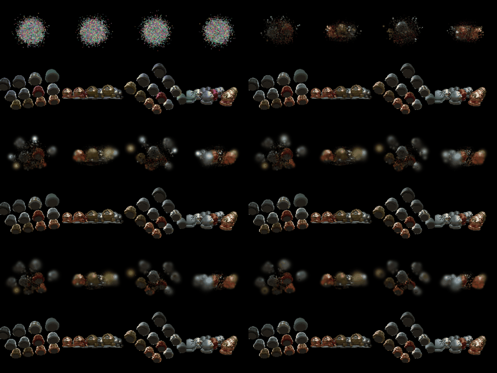
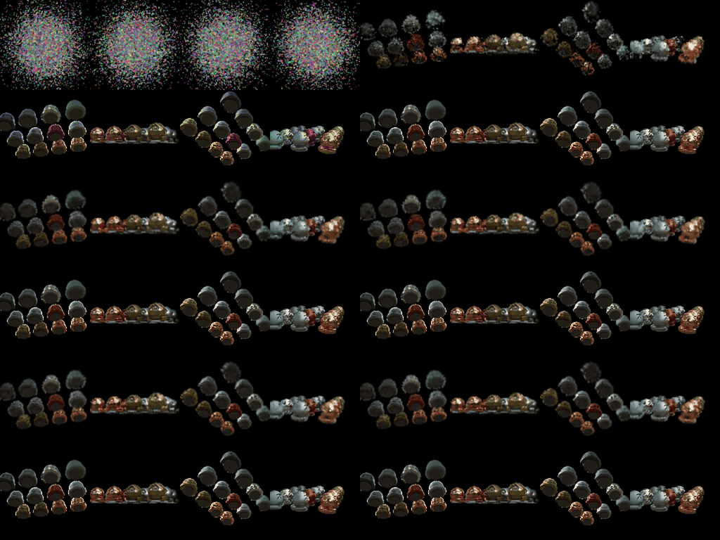


What I changed compared to Q6, and why.
- Wider random initialization (biggest effect). The skeleton samples the means from
N(0, 0.2²), so almost all Gaussians start within 0.4 units of the origin, while the spheres inmaterialsspread out to about 1.2 units. Gradients only reach a Gaussian through the pixels it covers, so a Gaussian that sits in the middle gets no signal from a sphere at the edge of the scene and never travels there. Scaling the initial means by 2.5 (std 0.5) puts Gaussians near every object from the start. My first improved attempt without this change (same lr schedule, SSIM and anisotropy) only reached PSNR 18.73 / SSIM 0.727, so the other tricks barely help if the Gaussians cannot reach the objects. - Larger means learning rate with exponential decay. Q6 used 0.001 for the means, which was fine when the points already sat on the surface. Here they need to move, so I start at 0.005 and decay it by a factor of 0.1 over training (like the original paper’s schedule for positions). The large rate early on lets Gaussians drift to the right sphere; the small rate at the end stops them from jittering, which is what made the baseline renders blurry.
- L1 + SSIM loss. The paper’s loss
(1 - λ) L1 + λ (1 - SSIM)withλ = 0.2. L1 alone is happy with a blurry average colour; SSIM compares local structure, so it pushes for sharp sphere edges and the dark bottoms of the spheres. - Anisotropic Gaussians. With the quaternion trainable, a Gaussian can stretch to cover the lit top of a sphere or its dark rim instead of needing several round blobs. On its own this gave only a small gain (that is what my first attempt showed), but it is cheap.
- 2000 iterations instead of 1000. With random init the first few hundred steps are spent just moving Gaussians into place, so the scene needs more steps than Q6 before the colours and scales settle.
What is still wrong: the renders are soft and the metal highlights are missing. The remaining blur comes from Gaussians that are too big and too few in the right places. In future work, I can try using adaptive density control (splitting large Gaussians with big gradients, clone small ones, prune transparent ones).