Assignment 2: Single View to 3D
16-825: Learning for 3D Vision · Name: Zixin Guo · Andrew ID: zixinguo
Everything here comes out of main.py (fit, train, eval, analyze). Each run used one
A40 or A100 GPU through Slurm. The ResNet18 encoder is fine-tuned end to end from the RGB
images; --load_feat was not used. Unless stated otherwise a run is 30k iterations at batch
size 32 with Adam at 4e-4, chamfer and F1 use 1000 sampled points, and F1 is reported at
threshold 0.05 averaged over the 678 chairs of the test split (one fixed random view each).
1. Exploring loss functions
1.1 Fitting a voxel grid
voxel_loss is binary cross-entropy with logits: the source grid holds logits, the target is the 0/1 binvox grid, and F.binary_cross_entropy_with_logits averages over the 32³ cells. The source starts as uniform noise in [0, 1], which after the sigmoid is “everything slightly more than half full”, so its 0.5 iso-surface is empty and the first panel is blank. 10k Adam steps bring the loss to 0.067 and the iso-surface matches the target cell for cell.

1.2 Fitting a point cloud
chamfer_loss calls knn_points with K=1 in both directions and adds the two mean squared nearest-neighbour distances. 5000 points drawn from N(0, 1) collapse onto the chair within a few hundred steps (final loss 3e-4). A point that is far from everything is no point’s nearest neighbour, so the target-to-source term ignores it and the source-to-target term only pulls it with a gradient that Adam has long since normalised away. That blind spot of chamfer distance shows up again in Section 2.

1.3 Fitting a mesh
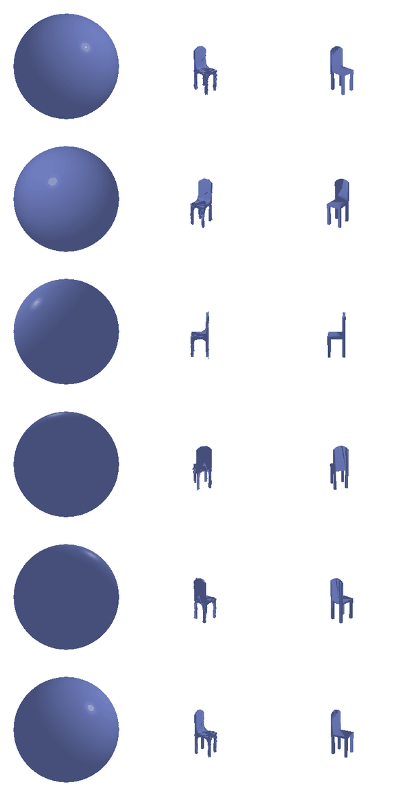
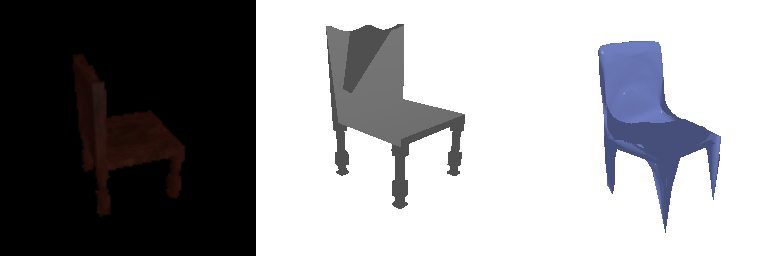
smoothness_loss is a uniform Laplacian regulariser. With L = mesh.laplacian_packed(), row i of L @ verts is the vector from vertex i to the mean of its neighbours; the loss is the mean norm of those vectors, zero on a flat patch and large on a spike. Chamfer on 5000 sampled points plus 0.1 x smoothness deforms ico_sphere(4) into the chair. As we can see, Back and seat are recovered cleanly; the legs stay webbed together at the bottom because a sphere cannot be torn into four tubes, only stretched.
The armchair and the plain chair come out as convincing
2. Reconstructing 3D from single view
All models share the ResNet18 -> 512-d feature encoder and differ only in the decoder
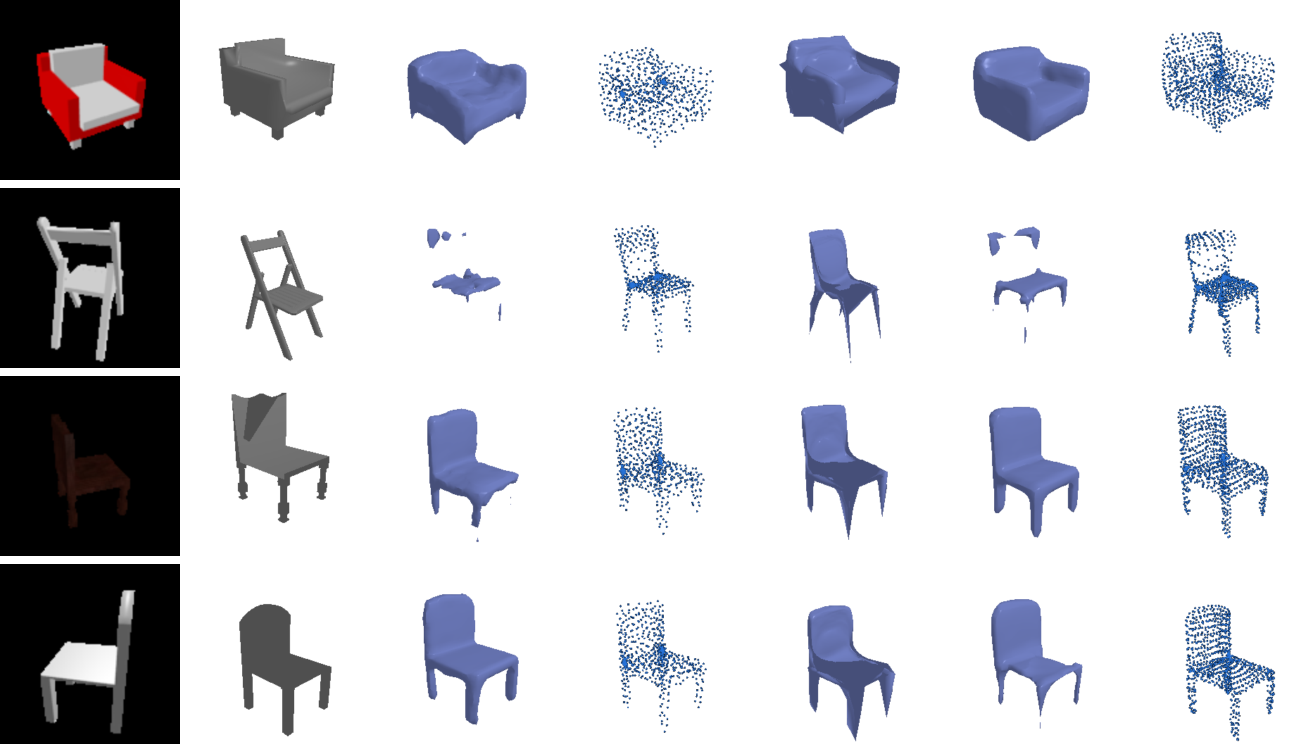
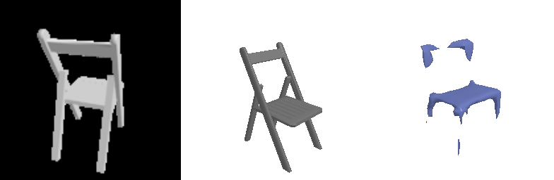
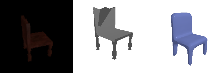
(model.py). Every panel below is input view | ground-truth mesh | prediction from the same fixed camera; the gifs turn the ground truth and the prediction together. Predicted voxel grids are thresholded at 0.5, meshed with marching cubes and moved into the mesh frame with the same transform the F1 code applies.
2.1 Image to voxel grid
Decoder. A linear layer maps the feature to a 256 x 2³ volume, four
ConvTranspose3d + BatchNorm + ReLU blocks double the side to 32 (channels 256-128-64-32-16) and a final 3x3x3 convolution gives one logit per cell, trained with the BCE from 1.1.
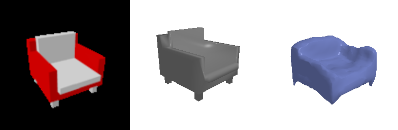



We can see the armchair and the plain chair show slightly inflated versions of the truth. The folding chair is the failure mode of this representation: every part of it is thinner than one voxel (1/32 of the bounding box), the network is unsure whether those cells are inside or outside, and apart from the seat and a few scraps of the back everything lands under 0.5.
2.2 Image to point cloud
Decoder. A 3-layer MLP 512 -> 1024 -> 2048 -> 3000 reshaped to 1000 x 3, trained with the chamfer loss from 1.2 against 1000 points freshly sampled from the ground-truth mesh every iteration.
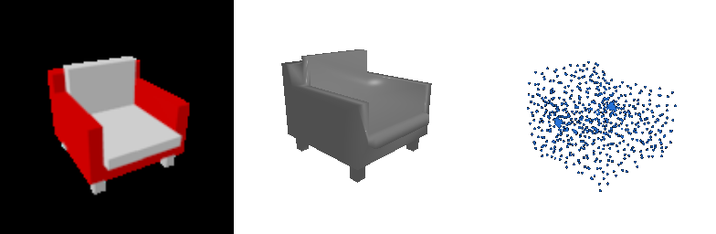
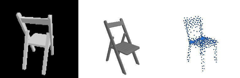
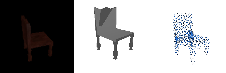
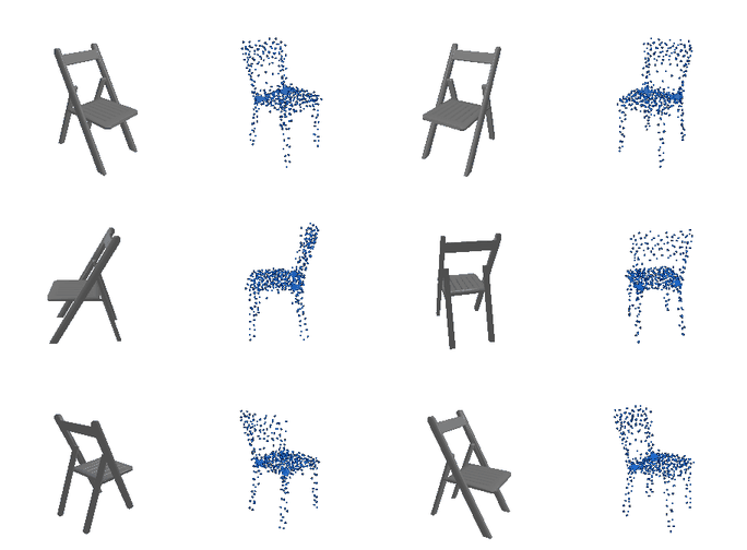
The clouds have the right silhouette for all three chairs, but they are fuzzy in a way that points scatter a little around every surface instead of sitting on it. Two dense knots also appear in the same place on every chair, a handful of output coordinates that the network has predicted at the average seat position and never moves; Note that in this case chamfer never punishes them because the seat is always there.
2.3 Image to mesh
Decoder. The same MLP as for points but its output is 2562 x 3 per-vertex offsets added
to ico_sphere(4). The last layer is zero-initialised so the very first prediction is the sphere itself and the network only learns the deformation. The loss is chamfer on 1000 points from each mesh plus 0.1 x the Laplacian smoothness of 1.3.
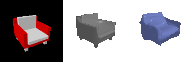
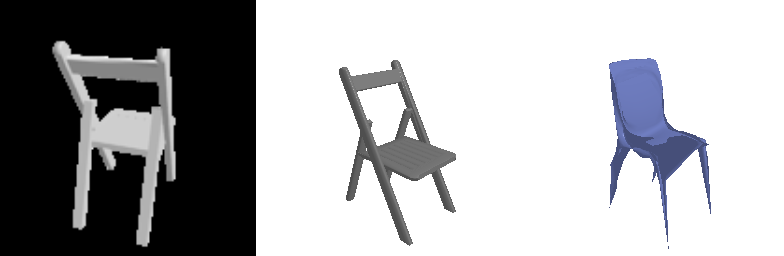
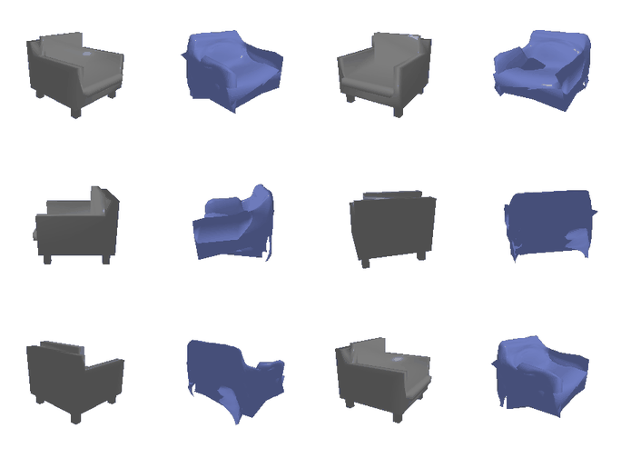
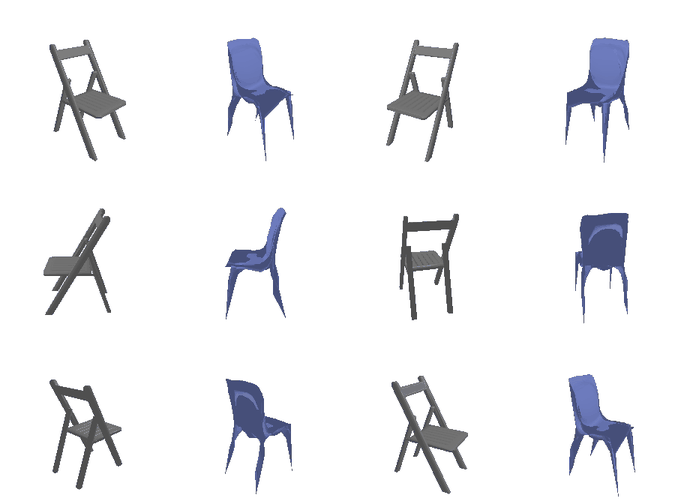
The meshes read as chairs from every angle and have proper seats, backs and legs, but the surface shape is messy. We can see a sphere has one connected sheet, so making four legs and a hole under the seat means folding that sheet back on itself, and the folds show up as creases and flaps. The armchair, which is nearly convex, appears to be the cleanest of the three.
Comparison.
| representation | F1@0.01 | 0.02 | 0.03 | 0.04 | 0.05 | precision@0.05 | recall@0.05 |
|---|---|---|---|---|---|---|---|
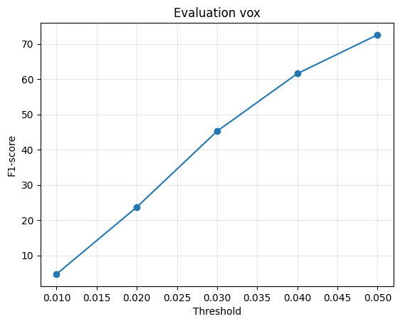
| voxel grid (2.1) | 4.7 | 23.7 | 45.2 | 61.6 | 72.6 | 74.3 | 73.0 |
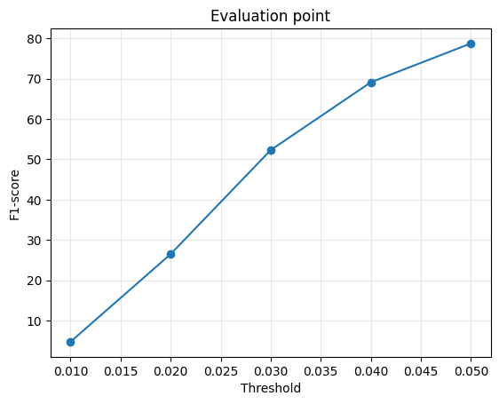
| point cloud (2.2) | 4.8 | 26.5 | 52.3 | 69.1 | 78.7 | 81.4 | 77.7 |
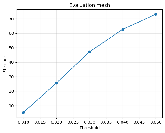
| mesh (2.3) | 5.2 | 25.6 | 47.1 | 62.6 | 73.1 | 72.3 | 74.6 |
Point cloud win, and mesh and voxels tie a few points behind. The ordering follows from how much each representation is allowed to do and what the metric can see.
- Point cloud. The 1000 points are completely free: no connectivity, no topology, no grid, and the training loss (chamfer) is essentially the same quantity F1 measures. The network can put a few points on each leg of the folding chair without having to explain how they connect to the seat. What it cannot do is produce a surface, and in this case F1 does not care.
- Mesh. The vertices are almost as free as points, but the surface between them must stay a deformed sphere. Chairs have holes (under the seat, between legs and back), so the sheet has to fold, and those folds put surface where there is none in the truth while the smoothness term keeps thin legs from stretching out fully.
- Voxels. A 32x32x32 grid caps the achievable accuracy before any learning happens: pushing the ground-truth voxel grids through the same marching cubes and F1 pipeline gives 79.3 on average. The trained model reaches 72.6. Its BCE loss is also the weakest match to F1 of the three. Most of the 32k cells are empty, so they dominate the loss; if the network puts a hesitant 0.4 on the cells of a thin leg it barely pays for it in BCE, yet the whole leg disappears once we threshold at 0.5.
So at this threshold the metric rewards freedom of placement over surface quality, and we see this is why the fuzzy point clouds score best and the visibly nicest voxel renders score worst.
2.4 Effects of hyper-parameter variations
Smoothness weight for the mesh decoder. I trained the mesh model with
w_smooth in {0, 0.1, 1, 10} (everything else identical) and also swapped the template for
the much coarser ico_sphere(2) (162 vertices instead of 2562).
| mesh run | F1@0.05 | precision | recall |
|---|---|---|---|
| w_smooth = 0 | 74.7 | 73.6 | 76.5 |
| w_smooth = 0.1 (2.3) | 73.1 | 72.3 | 74.6 |
| w_smooth = 1 | 69.5 | 66.0 | 74.6 |
| w_smooth = 10 | 63.9 | 66.1 | 63.0 |
| ico_sphere(2), w_smooth = 0.1 | 70.1 | 70.3 | 70.6 |
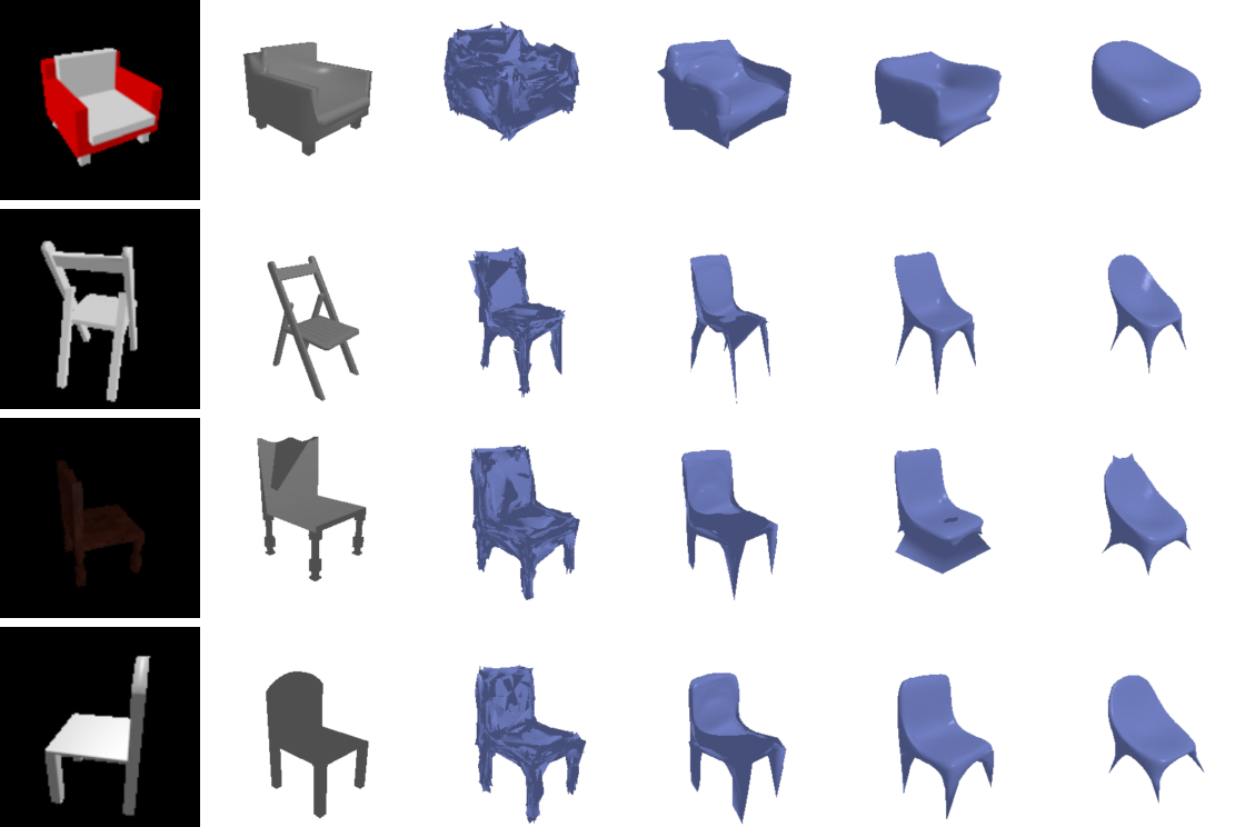
An interesting observation here is that the numbers and the pictures pull in opposite
directions. F1 is monotonically better with less smoothing: with w_smooth = 0 the
vertices go wherever chamfer sends them, so sampled points land on the true surface (recall
76.5, the best of any mesh run), but the mesh itself is a spiky shell. Raising the weight
trades that away: at 0.1 the creases are mostly gone and the legs stay separate, at 1 the
legs merge into a skirt, and at 10 every chair becomes the same smooth blob, so both
precision and recall drop. In short, w_smooth trades score for surface quality, and 0.1
is a reasonable middle.

The coarser template loses 3 F1 points: with 162 vertices a leg is only a couple of
triangles, so the network can only pull out four blunt cones. It does come out smoother at
the same w_smooth, since each Laplacian neighbourhood now spans a larger distance, which
makes fewer vertices a cheaper route to a smooth-looking mesh than a large smoothness weight.
2.5 Interpreting the model
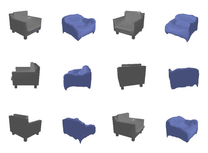
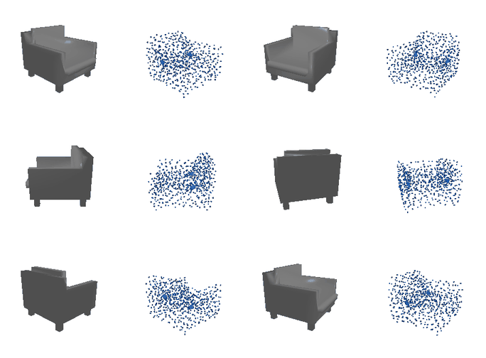
How much does the prediction depend on the view? Each test chair has ten renderings and the F1 above uses one of them at random. To see how much that choice matters, I ran the point and voxel models on all ten views of four test chairs and scored every prediction against the same ground truth.
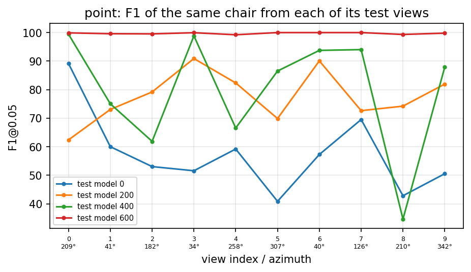
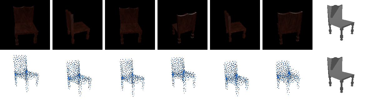

The spread is large. For both models the gap between the best and worst view of the same chair is about 36 F1 points on average, so a good part of the per-example variance in the test score comes from the view rather than the chair. The losing views are the low and back-facing ones where the seat is hidden; three-quarter views from slightly above, which is where most R2N2 renders sit, do consistently best, so the training viewpoint distribution shows directly in what the model is good at. The folding-chair strip also shows the voxel model hedging: two views give an almost empty grid, the rest give the seat and a few floating pieces of the back, and none give legs.
What is hiding under the 0.5 threshold? The evaluation only ever looks at the 0.5 iso-surface of the predicted occupancy, so I rendered the same grids at several thresholds.
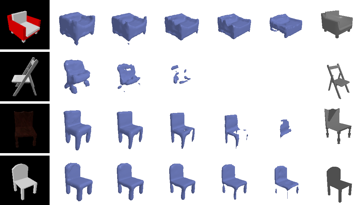
For the solid chairs the shape barely changes from 0.1 to 0.9; the network is confident about bulky parts. The folding chair is different: at 0.1 it is a complete, if fat, chair with legs, at 0.3 it starts to fragment, and at 0.5 only crumbs remain. So the model does know roughly where the chair is, it just gives the thin parts 0.2-0.4, which is the hedging that 2.1 and 2.3 blamed on the BCE loss. A per-shape threshold, or a loss that up-weights occupied cells, would recover most of it.
Does the encoder feature space mean anything? I took two test images, computed their ResNet features, linearly interpolated between them and decoded every intermediate feature with the mesh and point decoders.
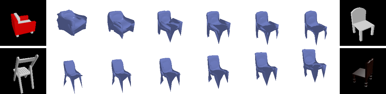
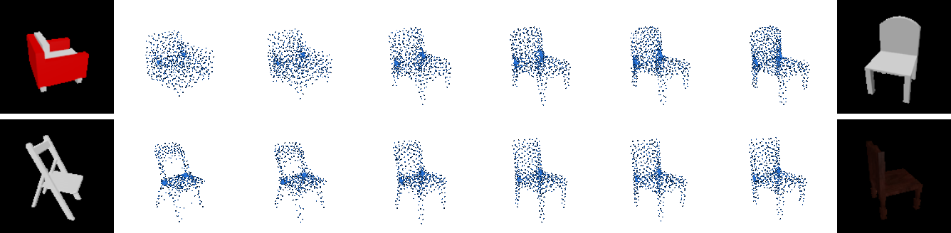
The walk is smooth and semantically sensible: the armchair loses its arms, grows a taller back and thinner legs, and turns into the dining chair with no collapse in between, and the point decoder produces exactly the same sequence of shapes. That tells me the decoders have learned a continuous shape space rather than a lookup of training chairs, and that the two decoders agree on what that space looks like. It also explains the failure cases: an unusual chair gets mapped to the nearest point on this smooth manifold of “typical chairs”, so the folding chair comes back as an ordinary four-legged chair with a solid seat.
3. Exploring other architectures / datasets
3.1 Implicit network
I replaced the voxel decoder with an occupancy network that predicts whether a queried 3D location is occupied, conditioned on the image. The image feature and query coordinates are each projected to 128 dimensions and added together. Three residual MLP blocks and a final linear layer produce one occupancy logit. I query a regular 32³ grid over the normalized coordinate range [-1, 1] and train with the same BCE loss and evaluation procedure as the voxel baseline.
The implicit decoder has 0.17M parameters, compared with 3.8M for the convolutional voxel decoder. Adding the projected features also avoids explicitly repeating and concatenating the 512-dimensional image feature at every query location.
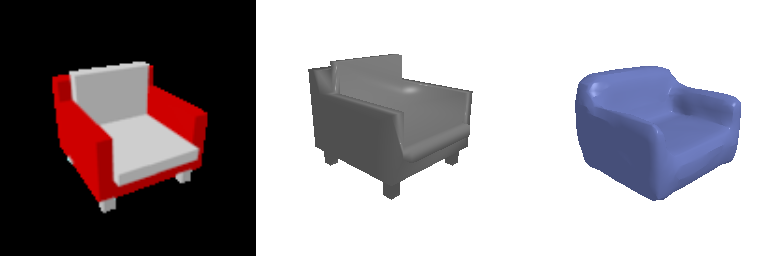
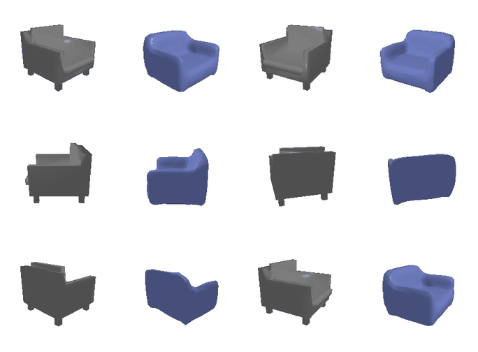
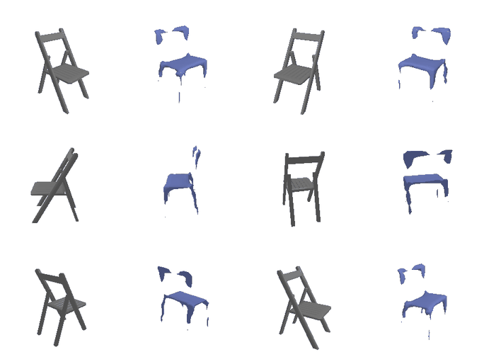
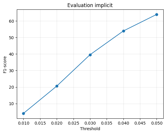
F1@0.05: 63.9, compared with 72.6 for the voxel baseline. Precision is 73.9 and recall is 61.8.
The reconstructions look smooth, but thin structures are often missing. In the folding-chair example, the prediction retains the seat while much of the frame disappears. This agrees with the lower recall. Under the current training budget, the smaller coordinate MLP captures less detail than the convolutional decoder. It can also be queried on a denser grid without changing its weights, although denser sampling alone would not recover geometry it has not learned.
3.2 Parametric network
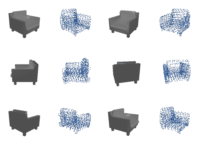
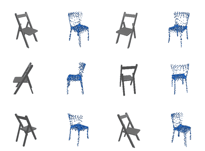
I used four AtlasNet-style patches to generate a point cloud. Each patch maps an image feature and a 2D coordinate (u, v) to a 3D point. The image feature and UV coordinates are projected to 256 dimensions, added, and passed through the patch MLP. Sampling 250 points from each patch gives 1,000 output points, supervised with the same Chamfer loss as Section 2.2.
Training uses new uniformly random UV samples each iteration. Evaluation uses a fixed set of 250 coordinates taken from a 16 × 16 UV grid. This makes the output deterministic, but regular spacing in UV does not guarantee uniform spacing on the 3D surface.
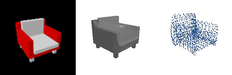
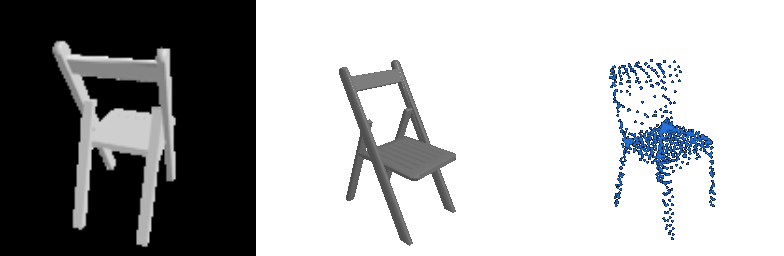
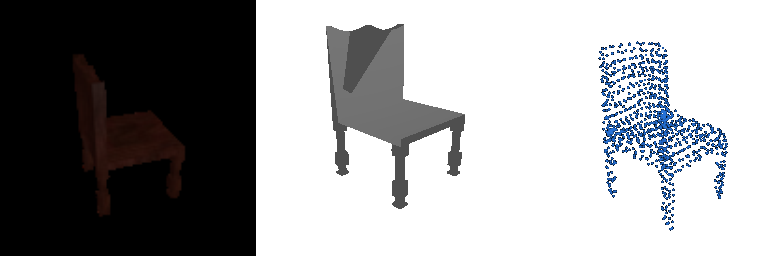
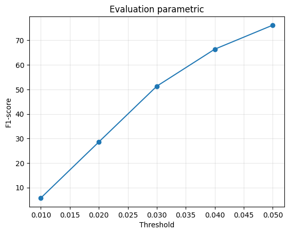
F1@0.05: 76.2, compared with 78.7 for the free-point decoder, using about 13× fewer decoder parameters (0.66M vs. 8.8M).
The predicted points form visible rows across the seat and back. Some patches also appear to stretch across gaps between the legs, placing points in empty space. This is consistent with the drop in precision from 81.4 to 75.0. Recall changes only slightly, from 77.7 to 78.1. The patches therefore offer a compact representation, but their continuity does not guarantee complete coverage or correct separation of nearby parts.
3.3 Extended dataset
I trained the point-cloud model using split_3c.json, with 6,100 chairs, 3,640 airplanes, and 3,146 cars. The decoder, batch size, and 30,000 training iterations were unchanged from Section 2.2. Both the chair-only and three-class models were evaluated on the same 1,451 test objects. The chair subset contains the same 678 objects used in Section 2.2.
| Training data | Chairs | Airplanes | Cars | All 1,451 |
|---|---|---|---|---|
| Chairs only | 78.7 | 68.8 | 69.5 | 73.5 |
| Chairs, airplanes, and cars | 79.8 | 96.3 | 93.8 | 87.9 |
F1@0.05 for the point-cloud model.
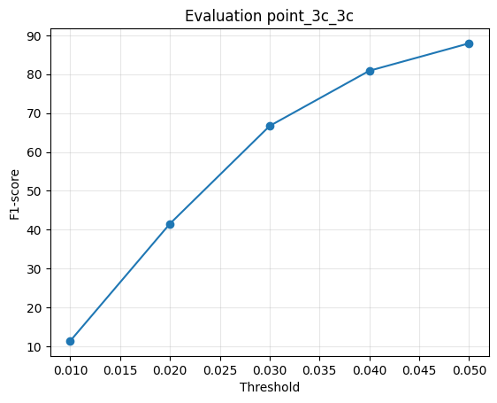


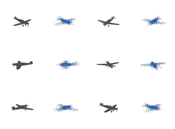
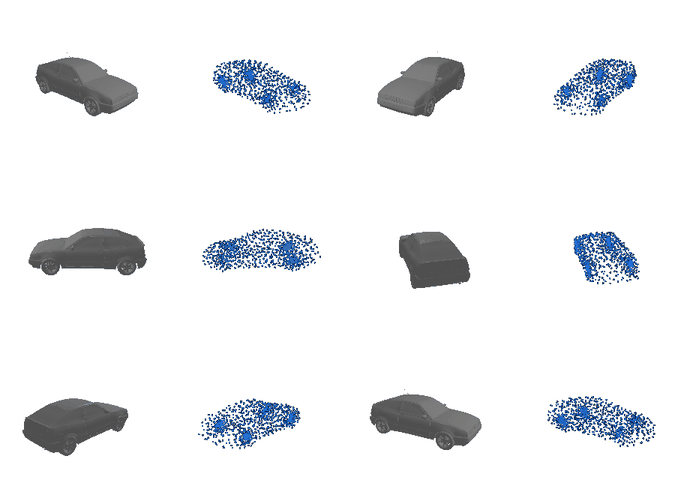
On the same test chairs, three-class training improves F1 by about one point. The chair reconstructions look similar, so the extra categories provide a small numerical gain without an obvious change in shape. Both models remain conservative on unusual chairs: the bench example becomes a broad seat with little distinct back structure. This single comparison suggests that adding categories did not hurt chair reconstruction, but does not establish a consistent improvement across training runs.
Across categories, the three-class model produces more distinct and recognizable shapes. Its airplane predictions share a fuselage-and-wing structure, and its cars share a body-and-roof structure. These examples show greater diversity between categories and consistent overall geometry within each category, while unusual instance details remain difficult. Most of the increase in the overall score comes from the much larger gains on airplanes and cars.
The chair-only model still scores around 69 on both unfamiliar categories, despite producing visibly incorrect shapes. F1 rewards nearby surface points, so partial geometric overlap can earn substantial credit without a semantically correct reconstruction. The qualitative comparisons help show errors that the single threshold score does not fully capture.