Assignment 3: Volume Rendering, NeRF and 3D Gaussian Splatting
16-825, Fall 2026 · Zijin Ye (Andrew ID: zijiny)
All results below were produced with the submitted code on an RTX 5070 Laptop GPU (8 GB).
1. Differentiable Volume Rendering
1.3 Ray sampling

vis_grid)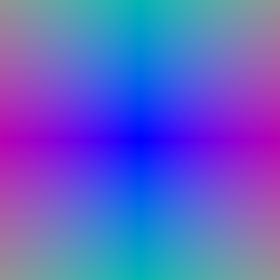
vis_rays)1.4 Point sampling
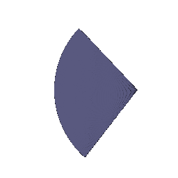
1.5 Volume rendering

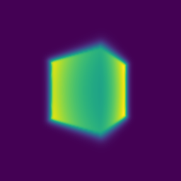
2. Optimizing a Basic Implicit Volume
Random ray sampling picks batch_size pixels with a random permutation of the pixel grid, and the loss is the MSE between rendered and ground-truth colors.
After training on train_box:
- Box center: (0.25, 0.25, -0.00)
- Box side lengths: (2.01, 1.50, 1.50)

3. Optimizing a Neural Radiance Field
Architecture. The 3D position is encoded with 6 harmonic frequencies (39 dims) and passed through a 6-layer, 128-unit ReLU MLP that re-injects the embedding at layer 3 (append_xyz: [3]). A linear layer followed by a ReLU predicts the density (non-negative), and a small 64-unit hidden layer followed by a sigmoid predicts RGB. Following the README, this model is not view dependent. It is trained with an MSE loss on 1024 random rays per step, 128 uniformly spaced samples per ray in [2, 6], for 250 epochs at 128×128.

4.1 View Dependence
Implementation (view_dependence: True in nerf_materials*.yaml). As in the NeRF paper, density depends on position only. The color head receives a 128-dimensional bottleneck feature from the position trunk, concatenated with a harmonic embedding of the normalized ray direction (2 frequencies, 15 dims), and maps it through a single 64-unit hidden layer to RGB. The direction enters only after the density has been computed, and only through one shallow layer. So it can modulate the color of a point (specular highlights, reflections), but it cannot change the geometry or memorize a separate appearance for every training view.
Results on materials (python volume_rendering_main.py --config-name=nerf_materials: 128×128, 250 epochs, lr 1e-4): 23.73 dB mean PSNR on the 200 held-out test views (evaluate.py). The metallic and glossy spheres show highlights that move across their surfaces as the camera orbits, which a position-only color cannot produce.


Comparison with the same model without view dependence (same seed and training settings; PSNR from evaluate.py):
| Model | Train views | Val views | Test views | Train − test gap |
|---|---|---|---|---|
| View-independent | 23.47 | 23.36 | 23.02 | 0.45 dB |
| View-dependent | 24.41 | 24.23 | 23.73 | 0.68 dB |

Trade-offs between view dependence and generalization. View dependence is needed for non-Lambertian materials: without it, a highlight that moves with the camera can only be explained by baking an average highlight into the surface color, or by inventing semi-transparent geometry (floaters) that reproduces it in the training views. However, every extra degree of freedom given to the direction lets the network fit the training views with view-specific colors instead of consistent geometry. With few or unevenly distributed views, a highly view-dependent model can reproduce each training image while producing wrong colors, or even wrong shapes "hidden" behind direction-specific color, from novel viewpoints. This is the shape-radiance ambiguity discussed in NeRF++. That is why the direction branch is kept low-capacity (few frequencies, one layer, after the density). Stronger view dependence (more frequencies, a deeper branch, the direction fed into the trunk) lowers the training loss but tends to hurt held-out views.
The measurements above show both sides of the trade-off on a small scale. View dependence improves every split, so this low-capacity branch generalizes. But the gain is largest on the training views (+0.94 dB) and smaller on novel test views (+0.71 dB), and the train-test gap grows from 0.45 to 0.68 dB. Part of the extra capacity is spent fitting view-specific appearance of the training images that does not transfer to new viewpoints.
4.2 Coarse/Fine Sampling
Implementation (configs/nerf_lego_coarse_fine.yaml):
CoarseFineNeuralRadianceFieldholds two independent NeRF MLPs with the same architecture as in Q3.- Coarse pass: 64 stratified samples per ray, each jittered uniformly within its bin during training (
perturb: True), rendered with the coarse network. - Importance sampling (
sampler.sample_pdf): the coarse weights define a piecewise-constant PDF over the bins between consecutive samples, and 128 new depths are drawn from it by inverse-CDF sampling (random quantiles while training, evenly spaced at test time). - Fine pass: the fine network is evaluated on the sorted union of coarse and fine depths (192 samples) and produces the final color and depth.
- Loss: MSE(coarse) + MSE(fine). Gradients do not flow through the sampling step, since the coarse weights are detached.
Density activation. With the ReLU density of Q3, training of this model got stuck: both networks rendered pure black from the first iterations and never escaped (their MSE equaled the error of an all-black image). This is the dead-ReLU failure mode on black-background scenes, and it also hit one unseeded materials run. For this experiment I therefore use a shifted softplus density, softplus(x − 1), as in mip-NeRF (density_activation: softplus); it cannot get stuck at zero. The single-network baseline below uses the same activation, so the comparison isolates the sampling strategy.
python volume_rendering_main.py --config-name=nerf_lego_coarse_fine
python volume_rendering_main.py --config-name=nerf_lego +implicit_function.density_activation=softplus   # baseline
| Lego, 128×128, 250 epochs | Test PSNR (200 views) | Parameters | Training step (1024 rays) | Render one 128×128 image |
|---|---|---|---|---|
| Single NeRF, 128 uniform samples | 25.73 dB | 101k | 31.4 ms | 144 ms |
| Coarse/fine, 64 stratified + 128 importance samples | 25.99 dB | 202k | 54.1 ms (1.7×) | 312 ms (2.2×) |
Timings are from benchmark.py on an otherwise idle RTX 5070 Laptop GPU.


Trade-offs. Coarse/fine sampling concentrates the fine network's samples where the coarse pass found the surface, so most fine samples land on the object rather than in empty space. This improves quality (+0.26 dB here, with visibly crisper edges). It costs twice the parameters (two MLPs), 1.7× the training time and 2.2× the rendering time: each ray now needs 64 coarse and 192 fine network evaluations plus a sequential dependency between the passes, compared with 128 evaluations for the baseline. At this low resolution and with a tight depth range, 128 uniform samples are already about 0.03 units apart, so the baseline is not badly undersampled and the gain is modest. The benefit grows with resolution, larger depth ranges and thin structures, where uniform sampling either misses fine detail or needs many more samples. That is why NeRF uses hierarchical sampling instead of simply increasing the number of uniform samples. Stratified jitter of the coarse samples also helps by exposing the networks to continuous positions instead of a fixed grid, which reduces aliasing.
4.3 VolSDF
Implementation.
- Distance MLP: harmonic embedding (6 frequencies), then 6 layers of 128 units with Softplus(β=100) activations, then a linear output with no activation, since an SDF can be negative. A smooth activation keeps the eikonal gradients well-behaved. The network uses the geometric initialization of SAL/IDR, so it starts as the SDF of a unit sphere.
- Color MLP: takes the last hidden features of the distance MLP concatenated with the embedding, passes them through 2 layers (128 hidden units), and applies a sigmoid.
get_distance_colorshares the distance trunk between both outputs. - Eikonal loss:
mean((‖∇d(x)‖ − 1)²)on points sampled uniformly in the bounding box. - SDF → density (VolSDF Eq. 2): σ(x) = α Ψβ(−d(x)), where Ψβ is the CDF of a zero-mean Laplace distribution with scale β. This gives σ = α(1 − ½ed/β) inside the surface (d < 0) and σ = ½α e−d/β outside. I evaluate both branches through |d|, so
torch.wherenever sees an overflowing exponential, which would produce NaN gradients.
Intuition for α and β. α is the density of the solid interior: deep inside the object σ → α, and at the surface σ = α/2. It sets how quickly a ray becomes opaque once it enters the object. β is the width of the transition from empty space (σ ≈ 0) to solid (σ ≈ α) around the zero level set. Small β gives an almost binary, sharp density step at the surface; large β smears density into a thick shell on both sides of the surface.
1. How does high β bias the learned SDF? Low β? With high β, there is significant density in front of the true surface, so rays accumulate opacity and color before they reach the zero level set. The photometric loss is then satisfied by a fuzzy shell, and the zero level set is not forced onto the visible surface. It ends up offset and over-smoothed, and thin structures get washed out. With low β, density is concentrated at the zero level set, so the rendered surface and the SDF surface coincide and the bias becomes small. The cost is that density, and with it the gradient, is essentially zero away from the surface.
2. Is an SDF easier to train with low or high β? High β. The density is smooth, so many samples along each ray receive non-zero weight and gradients reach the SDF even where the current surface estimate is far from the true one. With low β, only samples within a few β of the current surface contribute. With a fixed number of uniform samples, a very thin shell can even fall between samples, so gradients are sparse and noisy and optimization stalls more easily.
3. Is an accurate surface more likely with low or high β? Low β, for the reason given in question 1. When β → 0, the density converges to α·1[d < 0], an exact indicator of the solid, and the depth at which a ray saturates converges to the SDF zero crossing. VolSDF's opacity error bound also shrinks with β. In practice a moderately small β, used together with the eikonal term, works best: the eikonal term keeps the field a proper distance function, so a small β still yields a well-defined surface.
Results
Best result: α = 33.3, β = 0.03 (α = 1/β, eikonal weight 0.02, 128 samples per ray, 250 epochs):
python -m volume_rendering_main --config-name=volsdf_surface renderer.alpha=33.3 renderer.beta=0.03


Default settings, for comparison: α = 10, β = 0.05


Why these settings work better. With the default β = 0.05, the color renders are already good, but the extracted surface has a bloated "skirt" around and below the base plate. In that region the density is spread over a wide band, so the photometric loss is satisfied by a thick, fuzzy shell. Some of that geometry is only ever seen against the black background (or never seen at all, since all cameras are in the upper hemisphere), so nothing pulls the zero level set onto the true surface. This is the high-β bias described in question 1. Lowering β to 0.03 makes the density step at the surface sharper, so the rendered surface must coincide with the SDF zero level set. The base plate becomes a crisp rectangle, and thin parts such as the bucket arm and the tracks are recovered better. Setting α = 1/β, as in the VolSDF paper, keeps the interior opaque enough that a ray saturates within roughly one β of the surface. I did not go lower than 0.03: with 128 uniform samples over [2, 6], the sample spacing is about 0.031, and much smaller β would let the density shell fall between samples (question 2). The geometric initialization and the eikonal term keep training stable at this β.
5. 3D Gaussian Rasterization
The rasterizer in GS/model.py is fully vectorized over the N Gaussians in a mini-batch:
- 3D covariance: Σ = R S Sᵀ Rᵀ, with R from
quaternion_to_matrix. In the isotropic case the quaternions stay at identity, so Σ = s²I. - 2D covariance: Σ′ = J W Σ Wᵀ Jᵀ, where J is the provided perspective Jacobian and W is the world-to-camera rotation. Means are projected with
transform_points_screen, and depth is the z coordinate in view space. - Gaussians are sorted by depth with
argsort, and those behind the camera (z ≤ 0) are dropped. - α = o·exp(P), with P the Mahalanobis power. Ti is the exclusive cumulative product of (1 − αj), starting from the previous mini-batch's transmittance.
- C = Σ ci αi Ti. Depth uses the same weights with zi in place of ci, and the mask is Σ αi Ti. The weighted sums are computed with
tensordot, so the (N, H, W, 3) product is never materialized.
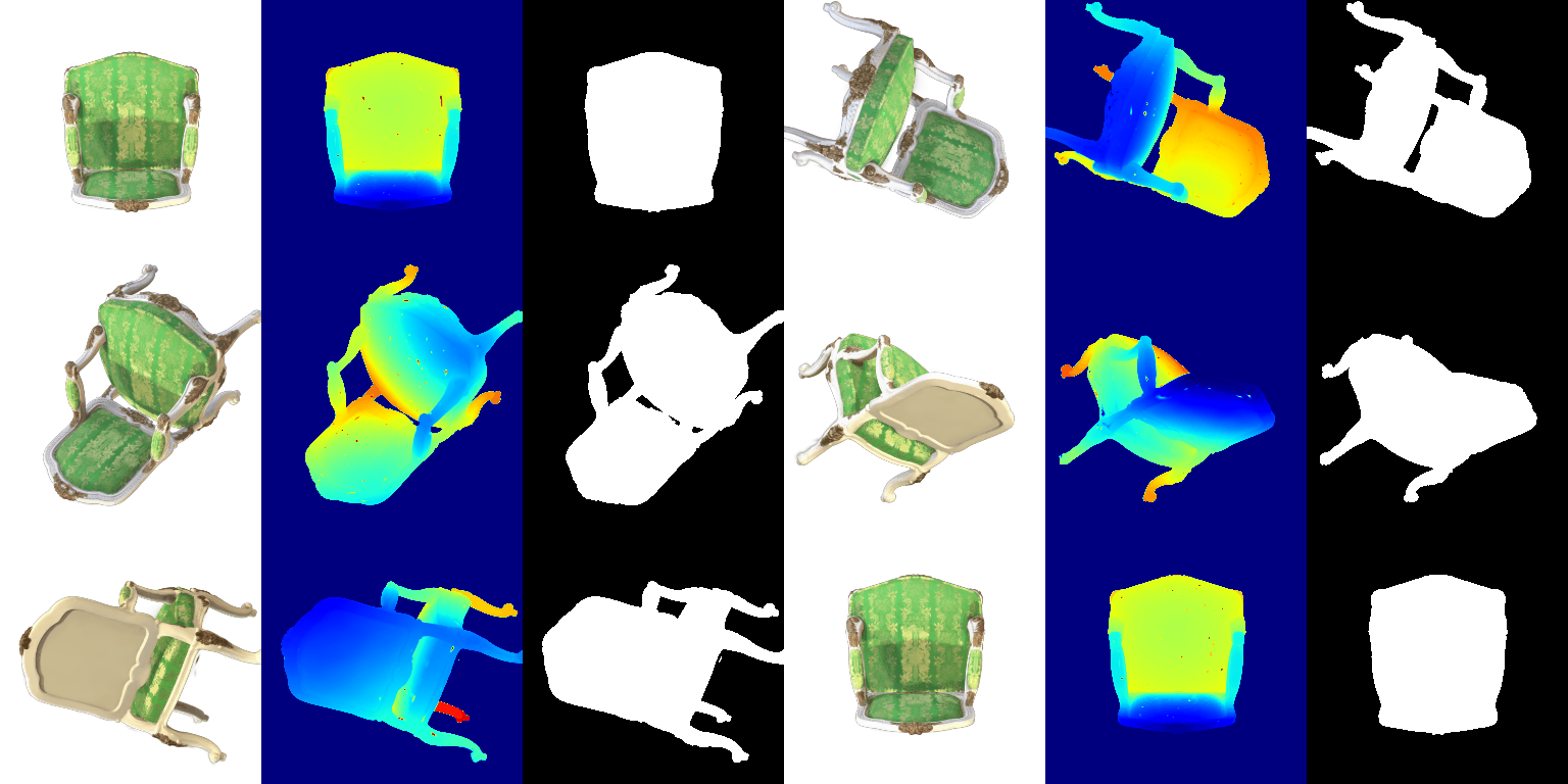
About the unit test. unit_test_gaussians.py reports 2/4. Tests 1 (3D covariance) and 3 (2D means) pass. Tests 2 and 4 fail because the reference values were computed with W = camera.R, while my code uses W = camera.Rᵀ. PyTorch3D uses row vectors (X_view = X_world · R + T), so the world-to-camera rotation in the column-vector form J W Σ Wᵀ Jᵀ is Rᵀ, not R. With W = R, every anisotropic Gaussian is rotated by the wrong matrix. The figure below shows the same three views rendered both ways: the unit-test convention (left) produces the hairy streaks that are also visible in the provided reference images, while Rᵀ (right) renders cleanly. Test 4 fails only because it reuses the 2D covariances of test 2. Changing that single line in compute_cov_2D back to camera.R makes all four tests pass.

6. Training 3D Gaussian Representations
make_trainable sets requires_grad on the means, scales, colors and opacities (plus the quaternions for anisotropic Gaussians). The optimizer is Adam with one parameter group per attribute. The forward pass renders the training view with Scene.render on a black background, and the loss is the L1 difference to the ground-truth image.
| Parameter | Learning rate | Reason |
|---|---|---|
| Opacities (pre-sigmoid) | 0.05 | Initialized at logit 8 (opacity ≈ 1); a large step size lets them drop quickly where Gaussians should be transparent. |
| Scales (log) | 0.005 | Log-space, so 0.005 is a ~0.5% relative change per step; larger values make Gaussians balloon. |
| Colors | 0.02 | RGB in [0, 1] starts random; it has to move fast but stay stable. |
| Means | 0.0005 | The point-cloud initialization is already accurate; the scene spans about 5 units, so this allows sub-pixel refinements without the points drifting. |
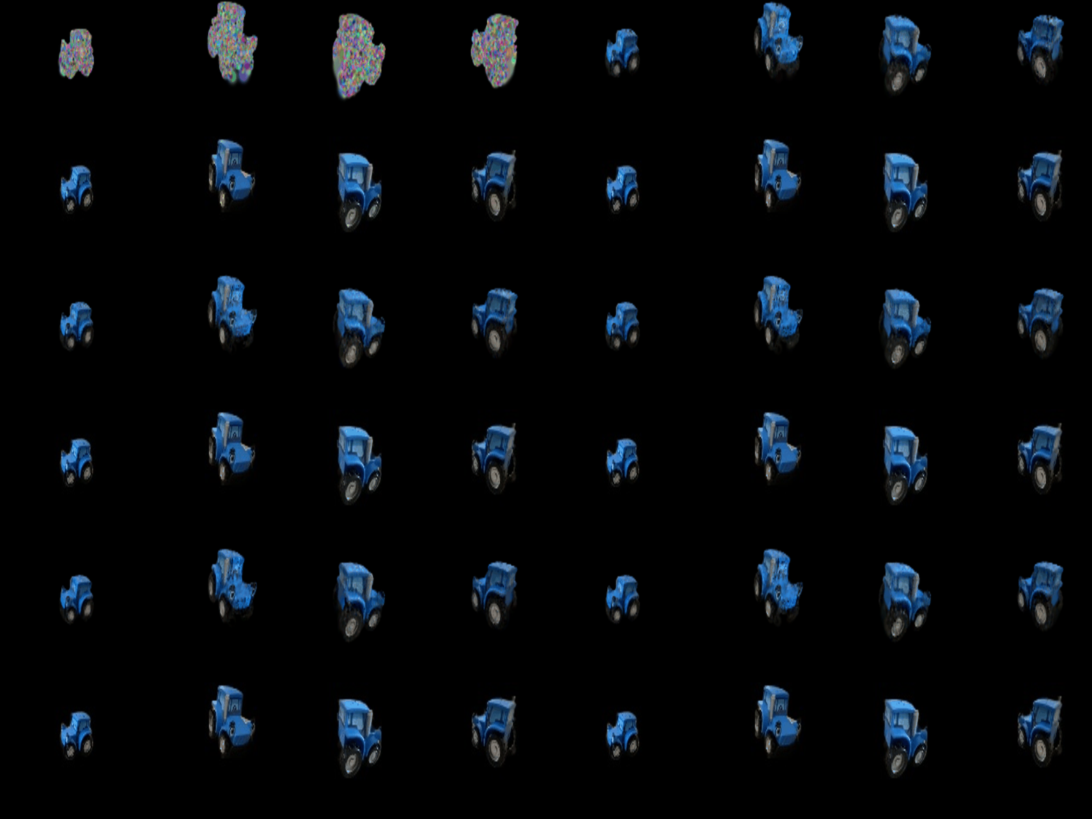
- Iterations: 1000, with one training view per iteration (
python train.py --gaussians_per_splat 2500) - Mean PSNR on the held-out views: 29.793
- Mean SSIM on the held-out views: 0.938

7.1 Rendering Using Spherical Harmonics
colours_from_spherical_harmonics evaluates the 16 real SH basis functions (degrees 0 to 3) for every Gaussian at once, as an (N, 16) matrix. Each basis value multiplies the corresponding RGB coefficients of the (N, 16, 3) SH tensor, and the results are summed, then offset by 0.5 and clamped at 0, exactly as in the original implementation. The view direction of each Gaussian is the normalized vector from the camera center (camera.get_camera_center()) to its mean. render.py --use_sh switches the renderer from the DC colors to these view-dependent colors.
Side-by-side comparisons (same view)


7.2 Training on a Harder Scene
Both setups are in GS/train_harder_scene.py:
cd GS
python train_harder_scene.py --baseline --num_itrs 1000 --gaussians_per_splat 2500   # baseline (Q6 setup)
python train_harder_scene.py --num_itrs 5000                                         # improved approach
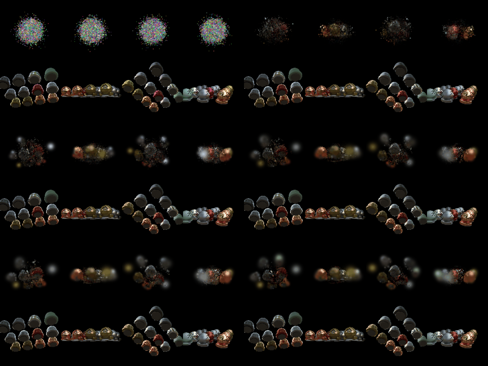
Baseline. Identical to Q6: 10,000 isotropic Gaussians with init_type="random" (means ~ N(0, 0.2²)), the same learning rates, L1 loss and 1000 iterations.
Modifications in the improved approach, compared to the Q6 setup:
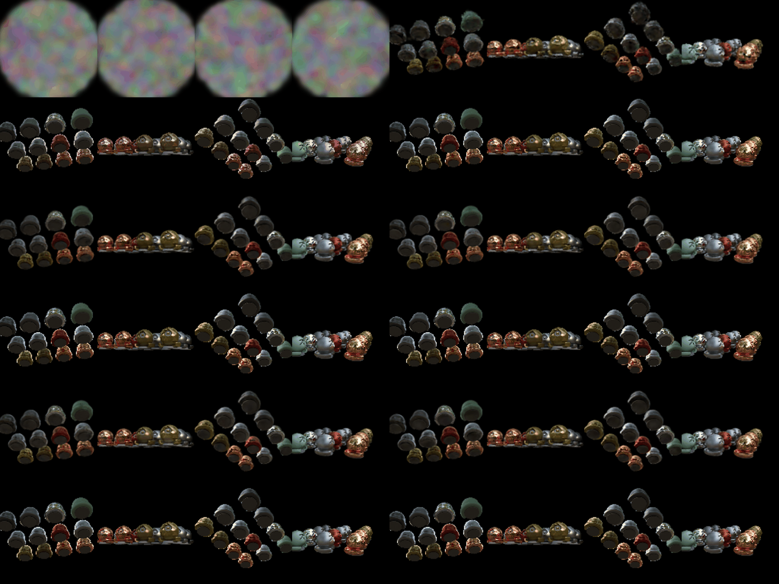
- Anisotropic Gaussians: per-axis scales and trainable quaternions (lr 0.001), so flat or elongated structure can be represented without many tiny isotropic blobs.
- Scene-covering initialization: still random, but the default N(0, 0.2²) puts every Gaussian in a small blob at the origin, while the materials spheres lie within about 1.3 units of it. I measured this extent by carving a 3D grid against the non-black foreground of the training images; only the radius was used, not the carved points. Means are therefore drawn uniformly inside a ball of radius 1.3, scales are set from the nearest-neighbor spacing, and opacities start at 0.1 instead of ≈1, so that early Gaussians do not occlude each other.
- Loss: 0.8·L1 + 0.2·(1 − SSIM), as in the original paper, using a differentiable SSIM with an 11×11 Gaussian window.
- Learning-rate schedule: the means' learning rate decays exponentially from 1.6e-3 to 1.6e-5 over training (large moves early, fine refinement late). The other attributes keep constant rates.
- Simplified adaptive density control (
DensityController): every 100 iterations between iterations 500 and 3000, Gaussians with a large average positional gradient are densified. Small ones are cloned; large ones are split into two samples drawn from the original Gaussian, with scales divided by 1.6. Nearly transparent (opacity < 0.005) or oversized Gaussians are pruned, capped at 40k Gaussians. Adam's moment estimates are carried over for surviving Gaussians. - Longer training: 5000 iterations.
- Tiled splatting (
Scene.splat_tiled), which makes the above affordable. Each Gaussian is evaluated only on the 16×16 tiles its footprint can reach, within radius √(2 ln(255·o) λmax), beyond which the template already zeroes α. Tiles are processed in groups with similar Gaussian counts (≤ 2²⁴ tile×Gaussian×pixel entries each), and each group is gradient-checkpointed, so memory stays bounded as densification adds Gaussians. The output is identical to the dense splat: on a test scene, images and all parameter gradients match to fp32 rounding (≤ 4e-5 against gradients up to 44), with one group or many.
Results
Learning rates. Baseline: the Q6 values (opacities 0.05, scales 0.005, colors 0.02, means 0.0005). Improved: opacities 0.05, scales 0.005, colors 0.01, quaternions 0.001, means 1.6e-3 decaying to 1.6e-5.
| Method | Iterations | Final #Gaussians | PSNR | SSIM |
|---|---|---|---|---|
| Baseline (Q6 setup, random init) | 1000 | 10,000 | 18.390 | 0.675 |
| Improved | 5000 | 39,919 | 25.117 | 0.911 |
Comparison. The baseline never recovers from its initialization. All Gaussians start in a small blob at the origin, and with isotropic Gaussians, a small learning rate for the means and no way to add Gaussians, they only spread a little. The progress GIF shows a blurry cluster of spheres in the middle of the frame, while the outer spheres are never reconstructed (18.4 dB). The improved approach covers the scene from the start and densifies wherever the reconstruction error is high. By the end, the renders match the ground truth closely, including the specular and patterned spheres (+6.7 dB PSNR, SSIM 0.675 → 0.911). The full 5000-iteration improved run, including the final renders and evaluation, took 28 minutes while sharing the GPU with another job. The dense baseline took 38 minutes for its 1000 iterations with 10k Gaussians.


Implementation notes
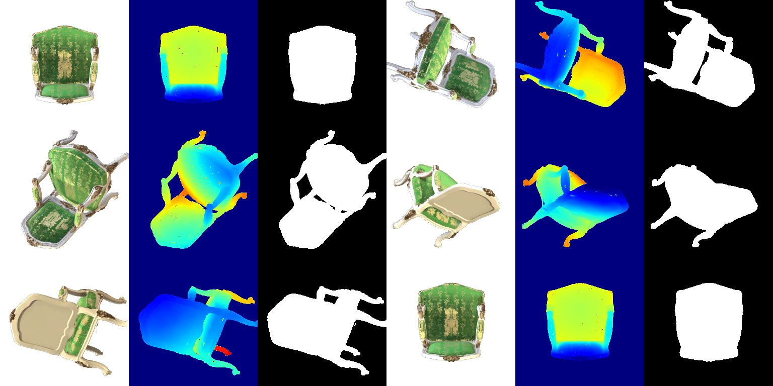
- Lego data. The PyTorch3D download URL in
nerf/dataset.pynow returns Access Denied.nerf/build_lego_dataset.pyrebuildslego.pth/lego.png(400 cameras, 100/100/200 split, 400×400 frames) from the original NeRF-synthetic Blender scene. Its Blender→PyTorch3D camera conversion reproduces the course-providedmaterials.pthto within 1.4e-6. - Environment. PyTorch 2.13 removed the
verboseargument of LR schedulers, so it is dropped increate_model.cfg.seedis now used to seed torch and numpy. One unseeded run of the view-dependent materials NeRF got stuck rendering only black (the failure mode discussed in 4.2); the seeded run (seed: 1) trains normally. - NeRF training script.
train_nerfalso checkpoints and renders after the last epoch. An optionaltraining.output_pathselects the output GIF, so different runs do not overwritepart_3.gif.nerf/evaluate.pyreports held-out PSNR andnerf/benchmark.pyreports timings. - Gaussian memory. In
Scene.render, each mini-batch splat is gradient-checkpointed when gradients are enabled. Otherwise autograd keeps every mini-batch's (per_splat, H, W) intermediates alive and mini-batching saves no memory, and training would need the ~15 GB quoted in the README. With checkpointing, truck training runs on an 8 GB GPU with--gaussians_per_splat 2500. The rendered values are unchanged. - Rotation convention. See the note in Q5 about
W = Rᵀand the unit test.