16-825 Assignment 2: Single View to 3D
Zijin Ye (Andrew ID: zijiny)
Losses, decoders and analysis for voxel, point cloud, mesh and implicit reconstruction on the R2N2 chair dataset.
--load_feat or CPU training for any part, including the extra-credit models.
Every model uses 4000 iterations at batch size 32 (batch size 16 for the implicit model), lr 4e-4, Adam. Chair evaluation covers all 678 test images; the three-class evaluation in 3.3 covers 1,451.
1. Exploring loss functions
1.1 Fitting a voxel grid
The loss is binary cross entropy on logits (F.binary_cross_entropy_with_logits), which applies the sigmoid inside the loss for numerical stability.
The optimized grid is shown on the left, ground truth on the right.

1.2 Fitting a point cloud
Chamfer loss is written from scratch using only knn_points. For every point it takes the squared distance to the nearest neighbour in the other cloud, averages each direction, and sums the two directions.

1.3 Fitting a mesh
The smoothness loss is the mean norm of the uniform Laplacian L·V, where each vertex is compared with the mean of its neighbours. It is combined with Chamfer on 5000 points sampled from both meshes (lr 4e-4, w_smooth 0.1, 10k steps, starting from an ico-sphere).


2. Reconstructing 3D from a single view
Every model shares a ResNet18 encoder that produces a 512-d global feature per image. Each panel below shows the input RGB | prediction | ground-truth mesh. The same three test images are used for every representation.
2.1 Image to voxel grid, F1@0.05 = 47.2
Decoder: a fully connected layer maps the feature to a 256×4³ grid, followed by three ConvTranspose3d + BatchNorm + ReLU stages (4³→8³→16³→32³) and a final 3×3×3 Conv3d that outputs occupancy logits.


Upper bound: feeding the ground-truth 32³ voxels through the same evaluation gives F1@0.05 = 77.2. The voxel model therefore reaches about 61% of what a 32³ grid can represent.
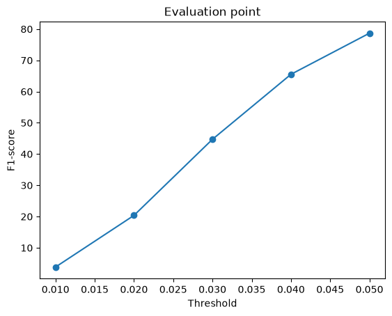
2.2 Image to point cloud, F1@0.05 = 78.7
Decoder: an MLP 512 → 1024 → 2048 → 1000×3 with LeakyReLU, trained with Chamfer loss against 1000 points sampled from the GT mesh.


2.3 Image to mesh, F1@0.05 = 70.7
Decoder: an MLP 512 → 1024 → 2048 → 2562×3 followed by tanh. It predicts a per-vertex offset of a level-4 ico-sphere. Training uses Chamfer on sampled points plus 0.1 × Laplacian smoothness.


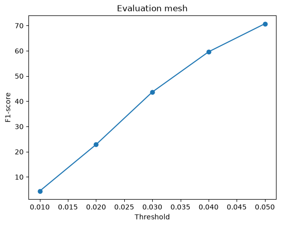
Comparison: voxel vs point vs mesh
| Representation | F1@0.01 | F1@0.02 | F1@0.03 | F1@0.04 | F1@0.05 |
|---|---|---|---|---|---|
| Voxel 32³ | 3.0 | 14.8 | 28.4 | 39.1 | 47.2 |
| Point cloud | 3.8 | 20.4 | 44.7 | 65.5 | 78.7 |
| Mesh | 4.4 | 22.8 | 43.7 | 59.6 | 70.7 |
- Point clouds score highest at 0.05 because the representation is unconstrained. Each point can go anywhere, and Chamfer directly optimizes the same nearest-neighbour distances that F1 measures. The model does not need to agree on topology or connectivity.
- Meshes win at tight thresholds (0.01–0.02) but lose at 0.05. A deformed sphere produces a continuous surface, so the points it does place lie on sharp sheets and are precise. But a genus-0 sphere cannot open the holes between chair legs or the gaps in a back rest, so whole regions stay unreachable and recall suffers at loose thresholds.
- Voxels score lowest. Resolution is the hard ceiling: a 32³ grid over the unit cube has cells about 0.031 wide (comparable to the 0.01–0.05 F1 thresholds), so even the ground-truth voxels only reach 77.2. On top of that, per-cell classification of mostly empty space makes the network conservative (see 2.5), so thin legs fall below the 0.5 iso-level and disappear.
2.4 Effect of the smoothness weight w_smooth
I trained the mesh model three times, identical except for w_smooth ∈ {0.01, 0.1, 1.0}. Besides F1, I measured surface quality on 100 test predictions: the mean Laplacian norm, the standard deviation of edge length, and the fraction of adjacent face pairs whose normals point in opposite directions ("folded" faces, a proxy for crumpling).
| w_smooth | F1@0.05 ↑ | Laplacian ↓ | Edge-length std ↓ | Folded faces ↓ |
|---|---|---|---|---|
| 0.01 | 74.2 | 0.0303 | 0.075 | 31.5% |
| 0.1 (Q2.3) | 70.7 | 0.0098 | 0.047 | 14.2% |
| 1.0 | 69.0 | 0.0043 | 0.023 | 3.5% |


Conclusion: w_smooth is a direct trade-off between the benchmark score and surface quality. Raising it 100× cuts folded faces by 9× (31.5% → 3.5%) and makes the surface 7× smoother, but costs 5.2 F1 points.
F1 only measures point-to-surface distance, so it rewards the crumpled solution: folding the sphere lets vertices reach into chair parts that a smooth genus-0 surface cannot cover.
The visual improvement is smaller than the numbers suggest because even the smoothest model still self-intersects. The Laplacian penalizes local roughness, not global folds.
To get meshes that are both accurate and clean, a regularizer that is not local (normal consistency, edge length) or a better initial topology would help more than tuning this weight.
2.5 Interpreting the models
(a) Where do the errors happen?
Left to right: input, predicted points coloured by their distance to the GT surface (precision error), and GT points coloured by their distance to the prediction (recall error). Blue means an error near 0 and red means 0.1 or more.
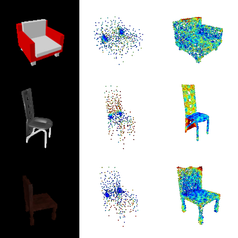
The recall errors (right column) are concentrated on thin, distinctive parts: the tall slotted back rest of chair 2 and the top of chair 3's back. The seat, which every chair has in about the same place, is reconstructed almost perfectly. The predicted clouds also show how the model hedges. When uncertain, it spreads points diffusely through the plausible volume, and it parks two dense clumps of points at the seat, where a point is always close to some surface. Chamfer loss makes this a cheap way to keep precision. To check that this is not a collapse, I scored the same predictions assigned to the wrong images: a constant prediction reaches only F1 55.2 and a shuffled one F1 59.5, against 78.3 for the real ones. The model clearly uses the image; the blur comes from single-view ambiguity.
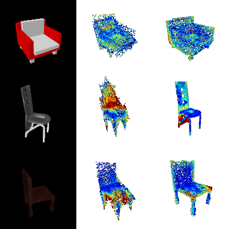
The mesh model fails in a different way. Its precision errors (middle column, red) sit on sheets of surface folded through empty space, such as in front of the seat of chair 2 and below the seat of chair 3. The sphere has to stretch past those regions to reach the legs, which is the crumpling measured in 2.4. The recall errors again sit on the thin, unusual parts, for example the curved sled base of chair 2.
(b) Is the learned shape space smooth?
I interpolated linearly between the ResNet features of two test images (the armchair on the left and the side chair on the right) and decoded each step.


The decoded shapes morph gradually from a wide, low armchair to a tall, narrow side chair: the back rises and the body narrows, with no sudden jumps. The dense "safe" clumps of the point model stay fixed at the seat throughout. The decoder has therefore learned a continuous shape manifold in which feature distance corresponds to geometric similarity, rather than memorizing separate shapes.
(c) How confident is the voxel model?
Columns: input, the mesh extracted at iso-levels 0.2 / 0.5 / 0.8, and the occupancy probability on the middle slice along each axis.

The 0.8 column is empty for every chair: the network never reaches 0.8 occupancy on these examples. The probability slices show that even the seat and back are only moderately confident (teal), with soft edges, and thin parts are fainter still. Most cells are empty and a single view is ambiguous, so BCE rewards hedging, and thin legs and armrests fall below 0.5. They appear at iso 0.2 and vanish at 0.5, which explains the missing legs in 2.1 and much of the gap to the 77.2 upper bound. Lowering the extraction threshold or weighting occupied cells more heavily in the loss would likely recover some of them.
3.1 Implicit network
Architecture: an occupancy MLP f(feature, xyz) → logit. The image feature and the encoded query point are each projected to 256-d and added, followed by four 256-d ReLU layers and one output. At inference it is queried on a 32×32×32 meshgrid over (−1, 1)³ and reshaped into a voxel grid, so it shares the voxel loss and evaluation.
| Model | F1@0.05 |
|---|---|
| Implicit, raw xyz input | 30.8 |
| Implicit, Fourier positional encoding (6 frequencies) | 36.4 |
| Voxel CNN decoder (2.1), for reference | 47.2 |
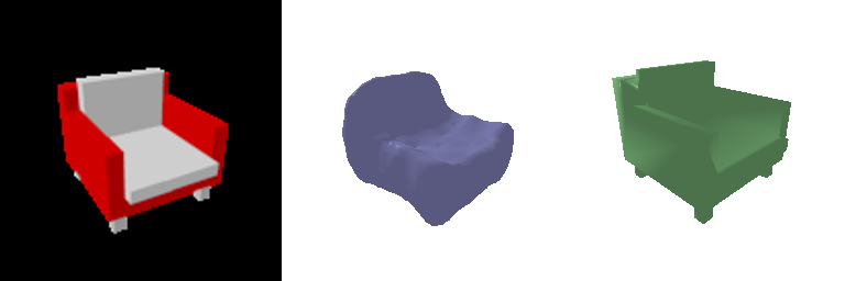
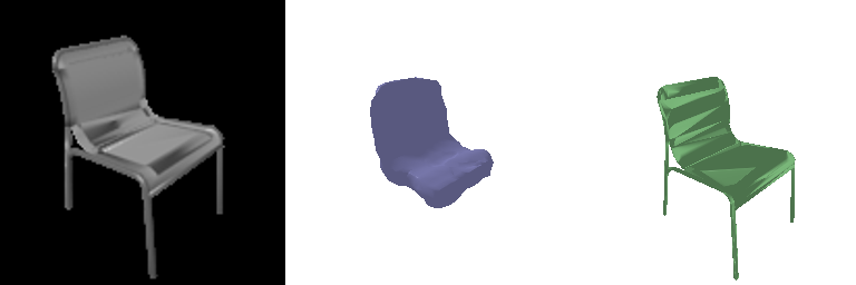
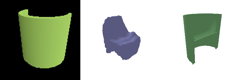
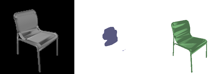
Analysis: my first version fed raw (x, y, z) into the MLP. It reached the same training BCE as the voxel CNN (about 0.09), yet at test time it produced a single blob (F1 30.8). An MLP on raw coordinates is biased toward very smooth functions ("spectral bias"), so it cannot represent a leg one or two voxels thick next to empty space. It hedges instead, predicting occupancy below 0.5 almost everywhere. Encoding the coordinates with sin/cos at 6 octave-spaced frequencies (as in NeRF and occupancy networks) lets the MLP represent sharp boundaries. The model then recovers the seat and back correctly and F1 rises to 36.4.
It still trails the voxel CNN (47.2) for three reasons:
- Memory limited it to batch size 16, since each image needs 32³ = 32,768 queries, so it saw half as many training examples. Its loss was still falling at the end of training (0.114 → 0.080 over the last 3000 iterations).
- Adding a single global feature gives every query the same conditioning. The 3D transposed-convolution decoder shares structure across neighbouring cells, which the per-point MLP has to learn from scratch.
- Legs are still missing, which is the same thin-structure hedging seen in 2.5(c).
The implicit form has a practical advantage the CNN lacks: resolution is chosen at query time. Training on random point subsets would remove the batch-size limit, and conditioning on local, pixel-aligned image features (as in PIFu) would likely close the gap.
3.2 Parametric network (extra credit)
Architecture (AtlasNet-style): K = 4 patches. Each patch is its own MLP fk(u, v, image feature) → (x, y, z), with layers 514 → 512 → 512 → 256 → 3, ReLU, and tanh output. During training, 250 points (u, v) are sampled uniformly from the unit square for each patch (1000 points in total), and the output is trained with the same Chamfer loss as 2.2. Same budget as 2.2: 4000 iterations on the GPU.
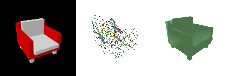
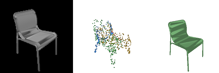

Points are coloured by the patch they come from.
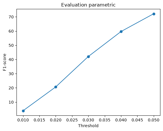
| Model (test samples) | F1@0.05 |
|---|---|
| Point decoder, 2.2 (fixed 1000 points) | 78.7 |
| Parametric, 1000 samples (training density) | 72.2 |
| Parametric, same model, 5000 samples* | 79.4 |
* Measured on every 4th test image (170 images), with the GT also sampled at 5000 points. Denser sampling on both sides also changes the metric, so this row shows what extra samples buy you rather than a like-for-like comparison with the point decoder, which can only ever output 1000 points.
What the parametric form gives
Left to right: input, 1000 samples, 10,000 samples from the same learned maps, and each patch's regular 24×24 (u, v) grid triangulated into a mesh.
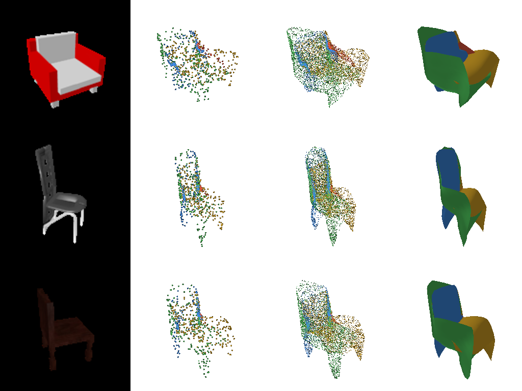
- The output is a continuous surface, not a point set. Because fk is a function of (u, v), the model can be sampled at any density after training. Triangulating the (u, v) grid gives a mesh for free, and these meshes are much cleaner than the ico-sphere deformations in 2.3. Each patch only covers part of the chair, so it does not have to fold one sphere around the whole object.
- At 1000 points it trails the free point decoder (72.2 vs 78.7). Each patch has to be a smooth image of a square, so it cannot scatter points in the diffuse "hedging" pattern that Chamfer rewards (see 2.5a). That constraint lowers the score at training density but produces far more structured shapes.
- The patches specialize on their own. blue covers the back rest, yellow the seat and side, and green the front and legs. The red patch has almost collapsed to a small region. This is a known AtlasNet failure mode, in which some charts become redundant; more patches or a coverage regularizer would help.
3.3 Extended dataset: training on three classes (extra credit)
Setup: the point cloud model from 2.2 was trained again, with identical architecture and hyperparameters and the same 4000 iterations at batch size 32 on the GPU. The only change was the training data: the three-class split (split_3c.json), with 12,886 training models (3,640 planes, 3,146 cars, 6,100 chairs) instead of 6,100 chairs.
Because the budget is fixed, the three-class model saw each chair about half as often. I then evaluated both models on the same chair test images, and both models on the three-class test set (1,451 models).
| F1@0.05 | Trained on chairs | Trained on 3 classes |
|---|---|---|
| Chair test set (same 678 images) | 78.7 | 77.9 |
| 3-class test set, all 1,451 | 74.2 | 86.1 |
| airplane (405) | 71.2 | 94.7 |
| car (368) | 70.1 | 91.6 |
| chair (678) | 78.4 | 78.0 |
Left to right: input, trained on chairs, trained on 3 classes, and ground truth. Rows show a plane, a car and a chair.

To measure the consistency and diversity of the outputs, I used 50 test chairs, each seen from 4 views:
| Chamfer (lower = closer) | Trained on chairs | Trained on 3 classes | GT chairs |
|---|---|---|---|
| Diversity: between predictions for different chairs | 0.0038 | 0.0037 | 0.0201 |
| View inconsistency: same chair, different views | 0.00079 | 0.00073 | – |
| Error: prediction vs. GT | 0.0039 | 0.0037 | – |
Analysis:
- Chairs barely suffer from sharing the model (78.7 → 77.9, −0.8 F1), even though the three-class model saw half as many chair images for the same budget. On the 50-chair subset, its Chamfer error is in fact slightly lower. A 512-d ResNet feature and an MLP decoder have more than enough capacity for three categories. The first thing the network has to decide, which category it is looking at, is easy from a single image, so the classes hardly compete.
- The chair-only model cannot represent anything but chairs. Shown a plane or a car, it still outputs its chair-shaped blob, with the dense seat clumps from 2.5a. It still reaches about 70 F1 on those classes, which again shows how forgiving F1@0.05 is for a blob placed in roughly the right volume. The three-class model produces flat, elongated wing-and-fuselage shapes and box-like cars, and scores 92–95 on them.
- Cars and planes are easier than chairs (94.7 and 91.6 vs 78.0), even though they were not seen more often. Within their category they vary much less: most cars are the same box with wheels, and planes are a fuselage with wings in a similar layout. Chairs have many topologies (legs, sled bases, armrests, slats) that one view does not pin down, so the model hedges on them the most.
- Diversity within chairs is essentially unchanged (0.0038 vs 0.0037, 3% lower). Both models' chair predictions are about 5× less varied than real chairs (0.020). The collapse toward a mean shape found in 2.5 comes from single-view ambiguity combined with Chamfer, not from the training set, so adding cars and planes does not make the chair outputs more varied.
- Consistency across views improves slightly (7% lower view inconsistency). Training on more varied shapes seems to push the encoder toward features about the object rather than the viewpoint. The effect is small compared with the error, so I would not over-interpret it.