Assignment 1 — Learning for 3D Vision
Rendering basics with PyTorch3D: turntables, camera extrinsics, hand-built polyhedra, and three
ways of writing down the same torus. Every figure below is regenerated by run_all.py
into output/.
1.1 360-degree Renders (5 points)
36 cameras at distance 3 and elevation 0, with azimuth swept evenly over
[0°, 360°) using look_at_view_transform. The 360° frame is dropped so
the loop does not stutter.
The point light rides along with the camera instead of sitting at a fixed world position. The
starter code already does this for its single view — camera centre and light are both at
(0, 0, −3) — and keeping them together is what stops the far side of the cow from
going black halfway through the turn.

starter/render_360.py1.2 Re-creating the Dolly Zoom (10 points)
A subject of half-height h at the origin covers a constant fraction of the frame as
long as tan(fov / 2) = h / distance. Sweeping the field of view from 5° to 120° and
solving for the distance at each step cancels the change in focal length:
h        = 3 · tan(30°) = 1.732      # so distance == 3 when fov == 60°
distance = h / tan(fov / 2)
T        = [[0, 0, distance]]
Across the 40 frames the camera travels from 39.7 units away at 5° to 1.0 units away at 120°. The cow holds its size while the checkerboard behind it stretches out and swallows the frame.

starter/dolly_zoom.py2.1 Constructing a Tetrahedron (5 points)
A tetrahedron needs 4 vertices and 4 triangular faces.
The vertices are four alternating corners of the cube [−1, 1]³, which makes the
tetrahedron regular. Each face is wound counter-clockwise seen from outside, so every face normal
points away from the centre:
vertices = (1, 1, 1), (1, −1, −1), (−1, 1, −1), (−1, −1, 1)
faces    = (0, 1, 2), (0, 3, 1), (0, 2, 3), (1, 3, 2)
These renders use a flat shader rather than the Phong shader in utils.py: with only
four vertices, per-vertex normals average across all three faces meeting at a corner and smear
the solid into a soft blob. One normal per face keeps the facets crisp.

starter/simple_meshes.py2.2 Constructing a Cube (5 points)
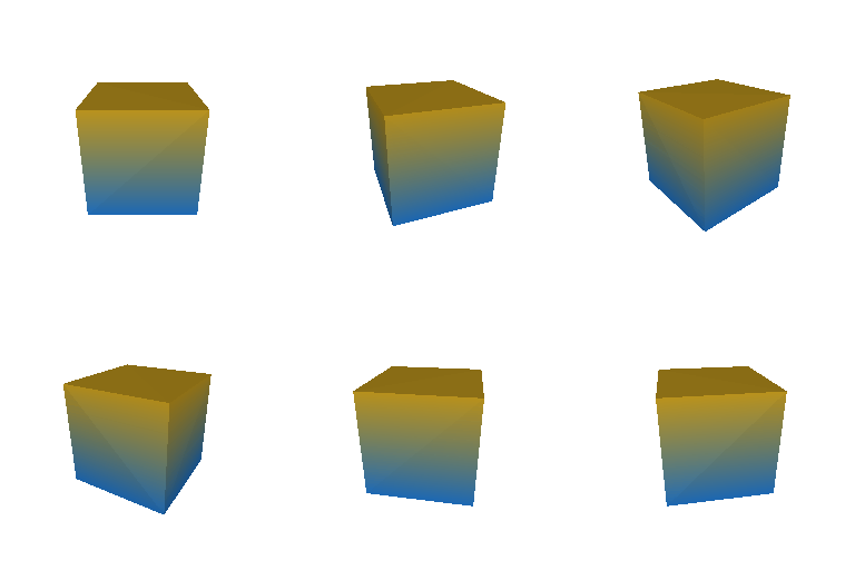
A cube needs 8 vertices and 12 triangular faces — two triangles per square side.
The eight corners of [−1, 1]³, with each square side split into two triangles
sharing a diagonal. As with the tetrahedron, all twelve triangles are wound counter-clockwise
from outside, so the six outward normals come out as ±x, ±y,
±z.
starter/simple_meshes.py3. Re-texturing a Mesh (10 points)
color1 = [0.0, 0.75, 1.0] — cyan, at the front of the cow (smallest z).
color2 = [1.0, 0.15, 0.55] — magenta, at the back (largest z).
Every other vertex is a linear blend of the two, weighted by where its z falls
between z_min and z_max:
alpha = (z − z_min) / (z_max − z_min)
color = alpha · color2 + (1 − alpha) · color1
The pair was picked for maximum separation in hue while keeping both ends bright enough to survive the Phong shading, so the nose-to-tail ramp stays readable from every angle in the turn.

starter/retexture.py4. Camera Transformations (10 points)
PyTorch3D maps world points into camera space with X_cam = X_world @ R + T. Two
consequences make each target image readable by inspection. First, row i of
R is where the world basis vector ei ends up in camera
coordinates. Second, an object at the world origin lands at exactly X_cam = T, so
T alone says where the subject sits in frame and how far away it is.
Camera space has +X pointing left in the image, +Y up and
+Z into the screen. Reading which way the coloured axis arrows point in each target
therefore pins down the rows of R directly, and the requirement that a centred
subject sits at T = (0, 0, 3) pins down T_relative. The arrows are red
for world +X, green for +Y and blue for +Z.
transform1 — roll the camera


The red arrow has swung from left to up and the green from up to right, so the whole image has
rotated 90° clockwise. That is the camera rolling −90° about its own optical axis. The camera
never moves, so T is unchanged.
R_relative = [[ 0, 1, 0],
              [−1, 0, 0],
              [ 0, 0, 1]]
T_relative = (0, 0, 0)
transform2 — orbit to a side view


Red has vanished (world +X now points into the screen) and blue points right, so the
camera has orbited 90° about the y axis. That rotation alone would send T to
(3, 0, 0) and push the cow out of frame, so T_relative pulls it back to
(0, 0, 3).
R_relative = [[ 0, 0, 1],
              [ 0, 1, 0],
              [−1, 0, 0]]
T_relative = (−3, 0, 3)
transform3 — dolly straight back


Orientation is untouched — the arrows point exactly where they did at the start — and the cow is half the size. Pure translation along the viewing axis, doubling the distance from 3 to 6. Note this is not a zoom: the field of view is unchanged, the camera physically moved.
R_relative = I
T_relative = (0, 0, 3)
transform4 — slide in the image plane


Same orientation, same size, but the cow has slid left and down. Because camera +X
is image-left and +Y is image-up, that is a translation of
(+0.5, −0.5, 0) — the camera moving right and up by half a unit.
R_relative = I
T_relative = (0.5, −0.5, 0)
These renders use data/cow_with_axis.obj so they line up against the targets arrow
for arrow. The same transforms applied to the plain data/cow.obj that
camera_transforms.py loads by default are in output/q4_transform_*.jpg.
5.1 Rendering Point Clouds from RGB-D Images (10 points)
Each image is unprojected with unproject_depth_image, which casts a ray through
every pixel and stops it at that pixel's depth. Two details needed handling first:
-
Zero-depth pixels. The masks admit many pixels whose depth is exactly 0 —
never actually observed. Unprojecting those divides by zero and produces
infandnancoordinates that drag the cloud's bounding box out to ±60 units. Intersecting the mask withdepth > 0removes about half the nominally-masked pixels from image 1. -
Handedness of the capture. The CO3D world frame has
+ypointing down, so a turntable built with the usualup = (0, 1, 0)renders the plant hanging from its pot. The cameras are givenup = (0, −1, 0)instead.

starter/rgbd_pointcloud.py
5.2 Parametric Functions (10 + 5 points)
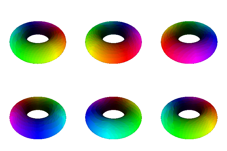
The torus is sampled on a 400 × 400 grid of (θ, φ) — 160,000 points — with major
radius 1.0 and minor radius 0.4:
x = (R + r·cos θ) · cos φ
y =      r·sin θ
z = (R + r·cos θ) · sin φ
Putting the axis of revolution along y rather than z is what keeps the
hole visible: a turntable sweeps azimuth, so a torus standing on the y axis presents the same
profile from every direction. The camera is tilted 40° above the plane of the ring, enough that
the near rim never covers the hole.

The new object: a trefoil knot
The second object sweeps a circle of radius 0.28 along the trefoil
c(t) = (sin t + 2 sin 2t, cos t − 2 cos 2t, −sin 3t), sampled at 600 points along
the curve and 90 around each ring. The circle needs a frame to live in, and the textbook Frenet
frame flips wherever the curve's curvature vanishes. Instead the normal is parallel
transported: start with any vector perpendicular to the first tangent, then at each step
re-project the previous normal into the plane perpendicular to the new tangent. The tube comes
out with no twist and no pinch anywhere along the knot.
5.3 Implicit Surfaces (15 + 5 points)
The same torus, this time as the zero level set of a single function, recovered with marching cubes over a 128³ voxel grid:
F(x, y, z) = (√(x² + z²) − R)² + y² − r²
The grid spans [−1.55, 1.55] on each axis, leaving clearance around the
R + r = 1.4 outer radius so the surface closes instead of being cut by the boundary.
Marching cubes returns vertices in voxel index space, so they are mapped back onto the
coordinates the function was evaluated at before the mesh is built. The result is 37,856 vertices
and 75,712 faces.


The new object: Goursat's tangle cube
One line of polynomial,
x⁴ − 5x² + y⁴ − 5y² + z⁴ − 5z² + 11.8 = 0, produces eight lobes joined by twelve
necks — a genus-5 surface. That is the argument for implicit representations in one image: the
topology is nowhere in the formula, it falls out of the level set, and writing the same object
down as an explicit mesh by hand would be miserable.
Mesh vs. point cloud: the trade-offs
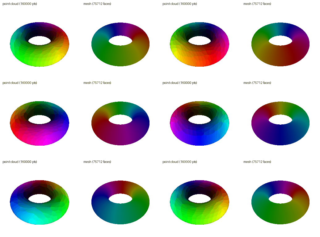
Both representations of the identical torus, rendered along the identical camera path:
| Point cloud | Mesh | |
|---|---|---|
| Primitives | 160,000 pts | 75,712 faces |
| Construction | 0.026 s | 0.105 s |
| Render, GPU (per frame) | 17.4 ms | 12.8 ms |
| Render, CPU (per frame) | 29.8 s | 10.8 s |
| Geometry in memory | 3.66 MiB | 1.73 MiB |
- Rendering speed. On the GPU the two are within a few milliseconds of each other and neither is the bottleneck. On the CPU the gap opens to nearly 3× in the mesh's favour, because compositing that many overlapping splats costs more than rasterising triangles that mostly cover a pixel or two each. Point rendering scales with the number of points times the splat area; mesh rendering scales with faces times screen coverage, and a good mesh needs far fewer primitives for the same surface.
- Rendering quality. The mesh wins outright. It is a continuous surface with real normals, so it shades smoothly, has a clean silhouette, and holds up under zoom. The point cloud has no normals at all — what looks like shading is just the colour assigned to each point — and its appearance depends on a splat radius that has to be retuned whenever the sampling density or the camera distance changes. Too small and the surface goes porous; too large and it turns to mush.
- Memory. The point cloud stores about twice the bytes for a visibly worse image. The mesh pays for connectivity — three indices per face — but that connectivity is exactly what lets it get away with so many fewer samples.
- Ease of use. Here the point cloud wins, and it is not close. Evaluate the parametric function on a grid, stack the results, done: no connectivity, no winding order, no watertightness. It also copes with things a mesh cannot — the RGB-D captures in 5.1 are partial, noisy, and of unknown topology, and turning them into a mesh is its own research problem. The implicit route needed a voxel grid (128³ is 2.1 million function evaluations, and roughly 98% of them land on cells the surface never passes through), a function that is genuinely signed, and a grid fine enough that thin features do not fall between samples.
- Where each belongs. Point clouds are the natural format for measured geometry — sensor output, partial views, anything accumulated incrementally. Meshes are the format for geometry you intend to light, texture, or simulate.
6. Do Something Fun (extra credit, 10 points)
A point cloud that morphs from the cow into a torus and back. The cow mesh is turned into 25,000 surface points with the stratified sampler from task 7; the torus is sampled from the parametric form in 5.2; and the two clouds are put into correspondence by sorting both by azimuth, so the transition unwinds instead of scattering.
Every frame interpolates position and colour between the matched pairs, then applies a twist
about the y axis whose angle is proportional to each point's height. The twist is scaled by
sin(πα), so it peaks halfway through and vanishes at both ends — the cow and the
torus are each seen undistorted. The blend factor follows
α = ½ − ½cos(2πt) while the camera makes exactly one revolution, which makes the
whole loop seamless.

starter/fun.py7. Sampling Points on Meshes (extra credit, 10 points)
Treating a mesh's vertices as a point cloud over-represents wherever the tessellation happens to be dense. Stratified sampling fixes that in three steps:
-
Pick a face with probability proportional to its area, computed as
½‖(v₁−v₀) × (v₂−v₀)‖and fed straight totorch.multinomial. -
Pick barycentric coordinates uniformly. Drawing
(u, v)uniformly from the unit square and folding the half whereu + v > 1back across the diagonal —(1−u, 1−v)— gives a uniform distribution over the triangle, with no rejection and no wasted draws. -
Evaluate
(1−u−v)·v₀ + u·v₁ + v·v₂.

starter/sample_points.py