Andrew ID: yunxianm
I hold out 10% of the 6,100 official training objects for validation (seed 825), leaving 5,490 training and 610 validation objects. Training samples one RGB view per object visit; validation and test use the lowest available view index. The figures show the first, middle, and last test objects: indices 0, 339, and 677.
All six experiments fine-tune an ImageNet-pretrained ResNet18 from RGB, without precomputed features. Training uses Adam, learning rate 0.0004, batch size 32, and 10,000 updates. Validation runs every 1,000 updates and selects the checkpoint with the lowest reconstruction loss. Mesh validation excludes the smoothing penalty.
Experiments use Python 3.11.10, PyTorch 2.4.1+cu124, and PyTorch3D on an A100 80GB GPU, with one seed and fixed batch/view order. The six training loops, including validation and checkpoint writes, took 41.0 minutes.
| Run | Training-loop time (minutes) | Selected checkpoint step |
|---|---|---|
| Voxel | 4.42 | 4,000 |
| Point cloud | 6.66 | 8,000 |
| Mesh, weight 0.1 | 8.48 | 3,000 |
| Implicit | 4.63 | 6,000 |
| Mesh, weight 0 | 8.48 | 7,000 |
| Mesh, weight 1 | 8.31 | 4,000 |
Validation losses fluctuate, with the best checkpoint occurring before the final update in every run. All test results use these validation-selected checkpoints.
I fit all three representations to training object
03001627/d8e2e2a923b372731cf97e154cc62f43 for 2,000 Adam steps at learning rate 0.01.
Each animation shows the optimized representation and target along the same
camera trajectory.
| Representation | Logged loss at step 1 | Logged loss at step 2,000 |
|---|---|---|
| Voxel BCE | 6.93147e-1 | 6.23100e-3 |
| Point Chamfer | 3.21540e-2 | 3.34300e-5 |
| Mesh Chamfer + 0.1 × smoothness | 3.16740e-2 | 7.23240e-4 |
Binary cross entropy optimizes 32 × 32 × 32 logits against binary occupancy targets. Marching cubes extracts the sigmoid probability surface at threshold 0.5.

Chamfer loss sums the mean squared nearest-neighbor distances in both directions.
The aggregation is implemented directly using knn_points. Both sets contain
2,000 points; source points start from a zero-mean Gaussian with standard deviation 0.2.

Vertex offsets deform a level-4 icosphere of radius 0.3 using sampled-point Chamfer plus 0.1 times uniform Laplacian smoothness. The regularizer averages each vertex's Euclidean distance to its neighbors' mean, then averages over meshes. The fitted mesh resembles the chair, but thin legs and connections show artifacts from deforming fixed sphere connectivity.

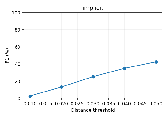
Evaluation covers all 678 test objects, with 1,000 points per representation and target. Points are sampled from ground-truth, mesh, and voxel surfaces; the point decoder outputs them directly. Sampling seeds are fixed per object. Precision measures the percentage of predicted points near a target point; recall reverses the direction. F1 is their harmonic mean, computed per object and then averaged. Thresholds are 0.01, 0.02, 0.03, 0.04, and 0.05; scores are percentages.
Voxel and implicit outputs use the starter's memory-to-reference conversion, 180-degree y rotation, and independent recentering of predicted and target samples. Points and meshes use direct coordinate comparison. The alignment therefore differs across representations. Visualizations use the same voxel orientation. Empty surfaces receive zero scores; non-finite predictions raise an error.
The decoder projects the 512-dimensional image feature to a 128 × 4 × 4 × 4 tensor. Three stride-2 transposed convolutions produce a 32³ logit grid, trained with BCE.
Test F1@0.05 is 41.43%. The seat and back are visible, but examples 339 and 677 lose most thin supports and openings. There are 82 empty predictions at threshold 0.5. Precision (57.76%) exceeds recall (36.29%), consistent with missing geometry. Background-dominated BCE and coarse resolution may contribute.


An MLP with hidden widths 512 and 1,024 outputs 3,000 coordinates, reshaped into 1,000 points. Bidirectional squared Chamfer compares them with samples from the target mesh.
Test F1@0.05 is 79.73%, the highest among the three base models. Independent point coordinates can represent separate chair structures without stretching a connected mesh between them. They also avoid the occupancy threshold used to extract voxel surfaces. This flexibility helps explain the higher F1. The examples capture the overall chair layout, though thin supports remain incomplete.


An MLP with a 512-unit hidden layer predicts offsets for the 2,562 vertices of a level-4 icosphere of radius 0.3. A zero-initialized output layer starts predictions at the template. Training combines Chamfer on 1,000 sampled points with uniform Laplacian smoothness weighted by 0.1.
Test F1@0.05 is 73.29%. The meshes capture parts of the seat/back layout but contain severe folds and protrusions. Chamfer rewards sampled points close to the target even when the triangles joining them form a folded surface.


Scores below are percentages at threshold 0.05; each column is averaged per object.
| Representation | Precision | Recall | F1 | Empty surfaces |
|---|---|---|---|---|
| Voxel | 57.76 | 36.29 | 41.43 | 82 |
| Point cloud | 80.63 | 80.98 | 79.73 | 0 |
| Mesh, weight 0.1 | 69.78 | 78.01 | 73.29 | 0 |
| Implicit occupancy | 56.18 | 37.88 | 42.64 | 106 |

The point model has the highest recall and F1. Mesh recall is higher than its precision, consistent with predictions covering target regions while also adding protrusions. Voxel and implicit models show the opposite pattern: precision exceeds recall, matching the missing supports and gaps in their renderings.
I compare smoothness weights 0, 0.1, and 1.0 while keeping the architecture, initialization seed, training steps, batch/view order, optimizer, and validation selection criterion fixed. Evaluation uses the same test objects and sampling seeds.
| Smoothness weight | Best validation Chamfer | Selected step | Test F1@0.05 (%) |
|---|---|---|---|
| 0 | 5.08100e-3 | 7,000 | 75.61 |
| 0.1 | 5.61900e-3 | 3,000 | 73.29 |
| 1.0 | 6.33900e-3 | 4,000 | 70.23 |

Test object 339, shown below with weights 0, 0.1, and 1:


Weight 0 has the highest F1 but many folds. Stronger smoothing removes some small folds while losing detail; sharp protrusions remain at weight 1. F1 falls by 2.32 percentage points from 0 to 0.1, then by 3.06 points from 0.1 to 1. None gives a clean surface for this thin chair.
I divide each of the three displayed test images into a 3 × 3 grid and replace one patch at a time with the ImageNet mean RGB color. Sensitivity is the mean Euclidean displacement of corresponding mesh vertices from the unmasked prediction, in source coordinate units. Patch indices start at zero in the upper-left corner.
| Test index | Most sensitive patch (row, column) | Maximum displacement | Minimum displacement |
|---|---|---|---|
| 0 | (0, 1) | 0.02619 | 0.01037 |
| 339 | (1, 2) | 0.03094 | 0.00510 |
| 677 | (0, 1) | 0.03734 | 0.00923 |


In example 0, masking the top-middle patch changes the mesh more than masking the middle-right patch. The mostly background top-left patch also causes noticeable movement. This suggests that the model responds to image context and the inserted mask as well as to the amount of chair area hidden.
Linear projections combine the image feature and a 3D query coordinate. A width-256 ReLU MLP predicts an occupancy logit. Training samples 4,096 indices per step from a normalized 32³ grid over [-1,1]³, using the corresponding voxel labels. Inference queries all 32³ locations in chunks, applies sigmoid, and extracts the 0.5 surface. Evaluation follows the voxel protocol.
Test F1@0.05 is 42.64%, 1.21 percentage points above the voxel model, with 106 empty surfaces at threshold 0.5. The coordinate-conditioned decoder produces smooth seat/back regions, but narrow supports and gaps remain missing. Its continuous form still uses the same voxel supervision and 32³ extraction grid, so it does not add finer geometric detail here. The higher mean F1 also comes with more empty surfaces than the voxel model.