Assignment 2: Single View to 3D
1. Exploring Loss Functions
1.1 Fitting a Voxel Grid

1.2 Fitting a Point Cloud

1.3 Fitting a Mesh

Losses. The voxel grid is fit with binary cross entropy on logits against the
target occupancy. The point cloud is fit with the symmetric Chamfer distance: for every source
point, the squared distance to its nearest target point (found with knn_points),
averaged, plus the same term from target to source. The mesh uses the same Chamfer distance
between points sampled from both surfaces, plus 0.1 times the uniform Laplacian smoothing loss,
which keeps each vertex close to the average of its neighbours so the surface does not fold.
2. Reconstructing 3D from a Single View
All models use a ResNet18 image encoder (512-d feature), batch size 32, learning rate 4e-4 and 10k iterations. Evaluation uses the 678 test chairs with one fixed view per object.
| Representation | Decoder | Decoder params | F1@0.05 |
|---|---|---|---|
| Voxel 32³ | Linear(512,512) → ReLU → Linear(512,32768) | 17.07 M | 54.74 |
| Point cloud, 1000 points | Linear(512,512) → ReLU → Linear(512,3000) | 1.80 M | 78.17 |
| Mesh, ico sphere level 4 | Linear(512,512) → ReLU → Linear(512,2562×3) | 4.21 M | 72.53 |
2.1 Image to Voxel Grid
F1@0.05 = 54.74


2.2 Image to Point Cloud
F1@0.05 = 78.17


2.3 Image to Mesh
F1@0.05 = 72.53


Comparing Voxels, Point Clouds and Meshes

As a reference for how much each representation loses on its own, I passed the ground truth itself through the same evaluation pipeline: the ground truth mesh sampled a second time for points and meshes, and the ground truth 32³ voxel grid (as ±10 logits) for voxels. This is a reference score, not a proven upper bound. A predicted grid with soft logits, for example, could place the surface between cells and score higher than the binarized ground truth.
| Representation | GT reconstruction reference | Model |
|---|---|---|
| Point cloud | 99.72 | 78.17 |
| Mesh | 99.72 | 72.53 |
| Voxel | 79.05 | 54.74 |

Ranking. Point clouds score highest (78.17), then meshes (72.53), then voxels (54.74).
Point clouds are the least constrained output. The decoder places 1000 points anywhere, the Chamfer loss it is trained with is close to what F1 measures, and nothing forces the points to form a connected surface, so thin legs cost nothing extra.
Meshes deform an ico sphere with fixed connectivity, so the output always has genus zero. Separate legs are not a problem for this topology, since a sphere can grow four protrusions. Only structures that actually form a closed loop or a through hole, such as an opening fully enclosed by the frame of the back, cannot be represented without tearing the surface. Even where the topology is fine, the vertices must travel far and unevenly from the sphere to reach thin legs, and a single linear layer predicts all 2562 offsets at once. The spikes, folded sheets and self intersections in the comparison figure come from these large deformations. Faces stretched across empty space produce sampled points away from the chair, which lowers precision.
Voxels lose accuracy before the model is even involved. Even the ground truth grid only scores 79.05 through this pipeline, because parts thinner than a cell either disappear or get thickened when the grid is turned back into a surface. The bench above is the extreme case: its own voxelization scores 22.0. On top of that, marching cubes on a coarse grid gives rounded surfaces, and the predicted probabilities are poorly calibrated for the fixed isovalue of 0.5 (see 2.4).
Representation versus model. For points and meshes the reference is 99.72, so nearly all of their gap to 100 reflects the model. For voxels the reference itself is only 79.05, so a substantial part of the low voxel score comes from discretization rather than from the model, and the raw comparison with points and meshes is unfavourable to voxels.
2.4 Effect of Hyperparameters
Mesh Smoothness Weight
| w_smooth | F1@0.05 |
|---|---|
| 0.1 (baseline) | 72.53 |
| 1.0 | 65.71 |


Raising w_smooth from 0.1 to 1.0 lowers F1 from 72.53 to 65.71, yet the meshes look
better. With the weak weight the prediction is covered in spikes and folded sheets. With the strong
weight it becomes a smooth, rounded shape that reads as one object, and the training loss also
decreased more steadily.
The Laplacian term penalizes every vertex that moves away from the average of its neighbours, and carving a chair out of a sphere needs exactly such large, local moves: pulling out four thin legs and leaving a thin back. A strong weight resists those moves, so the mesh settles into a rounded envelope around the chair. Its surface then passes through the empty space between the legs, which lowers precision, and it does not reach the feet, which lowers recall. The weak weight lets vertices go wherever the Chamfer loss pulls them, and F1 does not penalize the resulting self intersections because it only looks at sampled points. The metric therefore rewards the uglier mesh, and the right weight depends on whether the output will be used as a surface or only as a set of points.
Voxel Decoder Architecture and Extraction Isovalue
| Isovalue | MLP decoder (17.07 M) | 4 × ConvTranspose3d (3.81 M) |
|---|---|---|
| 0.3 | 65.46 | 64.86 |
| 0.4 | 63.98 | 59.19 |
| 0.5 (evaluation default) | 54.78 | 46.20 |

The default isovalue hides most of the difference. At the evaluation default of 0.5, the MLP decoder beats the ConvTranspose3d decoder by 8.6 points. At isovalue 0.3 the gap shrinks to 0.6 points, and both models improve a lot: the MLP by 10.7 and the deconvolution decoder by 18.7.
Calibration. Only about 3% of the cells in a target grid are occupied, so binary cross entropy pushes the predicted probabilities down, and cells near the surface of the chair end up below 0.5. Extracting the 0.5 level set therefore shrinks the shape and drops thin parts. A lower isovalue puts the surface back where the model actually places it. The deconvolution decoder is hurt more because more of its boundary cells fall between 0.3 and 0.5.
Architecture. Once the isovalue is chosen properly, the two decoders are almost equal, even though the deconvolution decoder has 4.5 times fewer parameters (3.81 M against 17.07 M). Sharing weights across space is a better use of parameters than a fully connected layer that predicts every cell independently. One caveat: the sweep was run on the test set, so 65.46 is slightly optimistic, and a fair choice of isovalue would use a held out split.
2.5 Interpreting the Model
Does the Prediction Depend on the Object?


For 50 test chairs, chosen at random with a fixed seed and shared by all three models, I measured the Chamfer distance from the prediction to its own ground truth and to the ground truth of 10 other chairs. If the model had only learned a generic chair, the two distances would be equal. The histograms show the difference, other minus own, for each chair. One voxel prediction was empty and is excluded, so the voxel averages use 49 chairs.
| Representation | To own ground truth | To other chairs | Ratio |
|---|---|---|---|
| Voxel | 0.0125 | 0.0164 | 1.31 |
| Point cloud | 0.0036 | 0.0074 | 2.06 |
| Mesh | 0.0028 | 0.0071 | 2.52 |
For point clouds and meshes the prediction is about twice as far from other chairs as from its own, and the histogram lies almost entirely right of zero, so the prediction does depend on the specific chair in the image. Voxels are the least specific, with a ratio of only 1.31, which matches their low F1.
Does the Prediction Stay the Same Across Input Views?


Mean pairwise Chamfer distance between predictions, with point clouds centered, on 5 chairs. Within a chair, I compare the predictions from all 10 available input views (45 pairs per chair). Across chairs, I compare the view 0 predictions of the 5 chairs (10 pairs). The ground truth meshes of the same 5 chairs differ from each other by 0.00754. The figures show 3 of the 5 chairs and 4 of the 10 views.
| Representation | Across views of one chair | Across different chairs | Ratio |
|---|---|---|---|
| Voxel | 0.00671 | 0.01914 | 0.35 |
| Point cloud | 0.00071 | 0.00197 | 0.36 |
| Mesh | 0.00112 | 0.00266 | 0.42 |
View invariance. For each chair I fed all 10 input views and compared how much those predictions differ with how much predictions for different chairs differ. The ratio is 0.35 to 0.42 for all three representations, so changing the viewpoint changes the output about a third as much as changing the chair. The encoder mostly captures the object, not the view.
Regression to the mean. The third column is the more revealing one. On these 5 chairs, predictions for different chairs are 3 to 4 times closer to each other (0.0020 for points, 0.0027 for meshes) than the real chairs are (0.0075). Five chairs is a small sample, so the factor is indicative rather than precise, but it suggests the model compresses the variety of chairs toward an average chair. This is what a Chamfer loss encourages when a single image is ambiguous: if the model cannot tell whether a hidden part is thin or thick, predicting something in between has the lowest expected loss. It also explains why the predicted point clouds in 2.2 look like soft blobs.
Voxels are the exception. Their spread across chairs (0.0191) is larger than that of the real chairs, and their spread across views of one chair is about ten times that of point clouds. This is unlikely to be diversity. Marching cubes on under-confident grids sometimes returns fragments or nothing at all (chair 1 in the comparison figure almost vanishes, and one of the 50 predictions in the specificity experiment was empty), and such broken surfaces are far from everything, which would inflate both distances.
3.1 Implicit Network
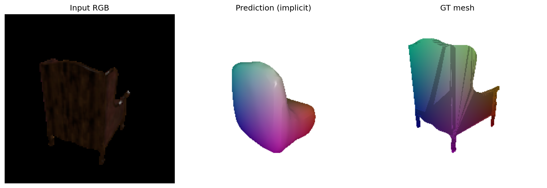
F1@0.05 = 31.28 at isovalue 0.5, and 52.61 at isovalue 0.3.
| Component | Setting |
|---|---|
| Query grid | 32³ points in [-1, 1]³ |
| Decoder | Linear(515,256) → ReLU → Linear(256,256) → ReLU → Linear(256,1) |
| Decoder params | 0.198 M |
| Loss | BCE with logits against the ground truth occupancy |
| Checkpoint shown | Step 4,500 (the other models are trained for about 10k steps) |


| Isovalue | 0.2 | 0.3 | 0.4 | 0.5 |
|---|---|---|---|---|
| F1@0.05 | 48.18 | 52.61 | 43.14 | 31.35 |


A smooth blob. The decoder receives raw (x, y, z) coordinates and applies a small ReLU MLP. Networks like this have a spectral bias: they fit low frequency functions easily and high frequency ones slowly. Occupancy is a step function that jumps from 0 to 1 at the surface, and the thin legs and back of a chair are exactly its high frequency part. The network learns the low frequency part, a smooth blob around the chair. It also has only 0.198 M decoder parameters and sees the image feature only once, at its input. Spectral bias is a likely cause of the smooth output but not the only possible one: this model was also trained for only 4,500 steps, less than half the budget of the other models, so it may be undertrained. A single run cannot separate the two.
Resolution does not help. Because the decoder is a continuous function of position, it can be queried at any resolution. Going from 32³ to 128³ multiplies the face count by 17, but the shape stays the same, because the learned function contains no detail to reveal. The bottleneck is the function, not the grid.
Isovalue. The calibration effect from 2.4 appears here too, and more strongly: F1 rises from 31.28 at isovalue 0.5 to 52.61 at 0.3. The 0.5 surface is too compact to reach the extremities of the chair, such as the top of the back and the feet. Lowering the isovalue grows the surface outward, from 11.6% to 17.0% of the cells, which brings it closer to those parts of the ground truth. Even so, the implicit model stays below the voxel MLP at its best isovalue (52.61 against 65.46), although with less than half the training. Positional encoding of the input coordinates is the standard fix for spectral bias and the natural next step.
3.2 Parametric Network
F1@0.05 = 74.50
| Component | Setting |
|---|---|
| Patches | 4, each maps (u, v) ∈ [0, 1]² to a 3D point |
| Per-patch MLP | Linear(514,512) → ReLU → Linear(512,256) → ReLU → Linear(256,128) → ReLU → Linear(128,3) → Tanh |
| Decoder params | 1.713 M |
| Sampling | 250 random (u, v) per patch, resampled at every forward pass |
| Loss | Chamfer distance, same as the point cloud model |


Score. The parametric decoder reaches 74.50, 3.7 points below the plain point cloud decoder (78.17), with a similar number of decoder parameters (1.71 M against 1.80 M). So the difference comes from the inductive bias rather than capacity. The point decoder can put each of its 1000 outputs anywhere. The parametric decoder produces each patch as a smooth function of (u, v), so a patch naturally forms a continuous sheet, and sheets are a poor fit for four separate thin legs.
What the patches learned. The patches do not divide the chair into clean parts. Patches 0, 1 and 2 overlap across the seat and back, with their points mixed together. Patch 3 is the exception: in all three examples it goes to the bottom of the chair, where the legs are. Nothing in the Chamfer loss asks the patches to share out the surface, so several patches can cover the same region at no cost. AtlasNet uses many more patches and trains much longer, which is likely why its patches look more like parts.
What it offers. Because (u, v) is resampled at every forward pass, the model can output any number of points at inference time without retraining, and each patch is a continuous surface that could be triangulated into a mesh.
3.3 Training on the Extended Dataset
Point cloud model, identical architecture and hyperparameters. Both checkpoints are taken at
step 9500 and evaluated on the same 678 test chairs with the same fixed views. The chair
entries of split_3c.json are identical to split_03001627.json, so no
filtering was needed.
| Training set | Objects | Epochs | F1@0.05 on chairs |
|---|---|---|---|
| Chairs only | 6,100 | 49.8 | 78.06 |
| Chairs, planes and cars | 12,886 | 23.6 | 79.49 |
The chair-only score here (78.06) is a re-evaluation with the same local code as the three-class model; its original evaluation gave 78.17. Evaluation itself is noisy: two runs of the same checkpoint differ by 1.16 F1 points per chair on average, although the signed differences cancel to +0.005 on the mean. The paired difference between the two checkpoints over the 678 test chairs is +1.42 (95% CI +0.36 to +2.49), well outside that noise. This compares these two specific checkpoints: each setting was trained once, so it does not capture variation between training runs.

Where the Difference Comes From
| Percentile of per-chair F1 | Chairs only | Three classes | Change |
|---|---|---|---|
| 5% | 32.36 | 42.07 | +9.71 |
| 10% | 48.73 | 57.42 | +8.69 |
| 25% | 71.86 | 75.78 | +3.91 |
| 50% | 84.55 | 84.45 | −0.09 |
| 75% | 91.18 | 90.60 | −0.58 |
| 90% | 95.05 | 93.95 | −1.10 |
| 95% | 96.43 | 95.11 | −1.32 |
| Chairs only | Three classes | |
|---|---|---|
| Chairs with F1 < 50 | 73 | 48 |
| Chairs with F1 < 60 | 106 | 74 |
| Standard deviation of F1 | 19.02 | 16.88 |

A small average gain with a clear pattern. Adding planes and cars to training raises the chair F1 by 1.42 points. The median barely moves, and the three-class model is better on only 49% of the chairs. The gain comes from the bottom of the distribution: the 5th and 10th percentiles rise by about 9 points, and the number of chairs below F1 50 falls from 73 to 48. At the top, typical chairs lose about 1 point.
Chairs that scored low improved most. Sorting chairs by their chair-only score, the worst fifth gains 14.6 points on average while the best fifth loses 4.0. This pattern should be read with care: whenever two models with imperfectly correlated per-chair scores are compared (here the correlation is 0.70), the chairs one model scored lowest tend to score higher with the other, even if neither model is better. The more reliable evidence is the distribution of scores itself, which does not depend on how chairs are paired: the three-class model has fewer severe failures (48 against 73 below F1 50), higher 5th and 10th percentiles, and a smaller spread. Chairs with unusual shapes change more in both directions (correlation 0.25 between how unusual a chair is and the size of the change), so an unusual shape alone does not predict improvement.
Interpretation. Planes and cars force the encoder to describe shape in more general terms than which kind of chair this is. The results are consistent with this broader shape prior avoiding the worst failures, at the price of some specialization: on ordinary chairs, the more specific prior of the chair-only model is slightly better. The three-class model gets this robustness while seeing each chair only half as often (23.6 epochs against 49.8); a run with matched epochs could widen the gain, but I did not run it.
Consistency and diversity. Across chairs the three-class model is more consistent: the standard deviation of F1 drops from 19.0 to 16.9, and severe failures become rarer. It is not more diverse. In the comparison figure both models still produce similar rounded clouds whatever the chair, and the three-class clouds are, if anything, more compact. This is the same pull toward an average shape found in 2.5, and adding classes does not remove it. Chair 493, a folding chair with thin crossed legs, shows the cost: the chair-only model matched it well (F1 90.1) and the three-class model did not (32.5).