

Yi Zhao · Andrew ID yizhao5
Everything below was produced by the code in the submitted zip, run on single GPUs of the lab cluster
(RTX PRO 5000 for Mini-LVSM, A100 for Mini-VGGT) on the full course data (224 training scenes; the prepared
validation and test splits with 28 scenes each). Numbers in the text are read from the run outputs. The cluster's
containers have a 64 MB /dev/shm, too small for PyTorch DataLoader worker processes, so batches are
loaded by threads instead (a4data/threaded_loader.py, opt-in); this changes only how fast samples are
produced, not which samples or how they are computed.
All five Q1 functions are implemented in a4data/geometry.py (vectorised, no loops). resize_intrinsics applies xout = s(xin + 0.5) − 0.5 per axis as a matrix A K; unproject_depth scales K-1[u, v, 1] by z-depth and maps it with the camera-to-world pose; canonicalize_cameras uses T0-1 Ti in float64 and the provided scene scale; camera_rays and plucker_coordinates follow the data contract. As an independent check, recomputing rays, Plücker coordinates and unprojected points from the TA-prepared validation cameras reproduces the prepared fields to 2.4e-7.


Same frames in both stages (fixed sampling, seed 825). The right-hand panel of each viewer prints the first camera center and the valid-point centroid distance.
python scripts/check_data.py --config configs/scannetpp/iphone/data.json --split train --max-samples 4
| sample | views | res. | valid depth | max point reproj. [px] | max ray reproj. [px] | centroid dist. |
|---|---|---|---|---|---|---|
| 260fa55d50_frame_001060 | 8 | 224 | 0.879 | 1.15e-04 | 8.22e-05 | 1.0000 |
| f6659a3107_frame_005010 | 8 | 224 | 0.966 | 1.11e-04 | 1.03e-04 | 1.0000 |
| 8be0cd3817_frame_005130 | 8 | 224 | 0.987 | 1.10e-04 | 1.02e-04 | 1.0000 |
| a980334473_frame_003080 | 8 | 224 | 0.912 | 8.63e-05 | 7.63e-05 | 1.0000 |
Full output of the command (JSON printed by check_data.py):
{
  "split": "train",
  "dataset_samples": 224,
  "checked_samples": 4,
  "samples": [
    {
      "sequence_name": "260fa55d50_frame_001060",
      "views": 8,
      "resolution": 224,
      "valid_depth_fraction": 0.8790407776832581,
      "max_reprojection_error_px": 0.00011475836799945682,
      "max_ray_reprojection_error_px": 8.217109279939905e-05,
      "centroid_distance": 1.0
    },
    {
      "sequence_name": "f6659a3107_frame_005010",
      "views": 8,
      "resolution": 224,
      "valid_depth_fraction": 0.9656234979629517,
      "max_reprojection_error_px": 0.00011108566104667261,
      "max_ray_reprojection_error_px": 0.00010327453492209315,
      "centroid_distance": 1.0
    },
    {
      "sequence_name": "8be0cd3817_frame_005130",
      "views": 8,
      "resolution": 224,
      "valid_depth_fraction": 0.9871004223823547,
      "max_reprojection_error_px": 0.0001100326917367056,
      "max_ray_reprojection_error_px": 0.00010235906665911898,
      "centroid_distance": 1.0
    },
    {
      "sequence_name": "a980334473_frame_003080",
      "views": 8,
      "resolution": 224,
      "valid_depth_fraction": 0.9118602275848389,
      "max_reprojection_error_px": 8.63167442730628e-05,
      "max_ray_reprojection_error_px": 7.62939453125e-05,
      "centroid_distance": 1.0
    }
  ],
  "batch_shapes": {
    "rgb": [
      2,
      8,
      3,
      224,
      224
    ],
    "depth": [
      2,
      8,
      1,
      224,
      224
    ],
    "depth_valid": [
      2,
      8,
      1,
      224,
      224
    ],
    "K": [
      2,
      8,
      3,
      3
    ],
    "frame_numbers": [
      2,
      8
    ],
    "T_world_from_camera": [
      2,
      8,
      4,
      4
    ],
    "original_world_from_reference": [
      2,
      4,
      4
    ],
    "scene_scale": [
      2
    ],
    "points_world": [
      2,
      8,
      3,
      224,
      224
    ],
    "ray_origins": [
      2,
      8,
      3,
      224,
      224
    ],
    "ray_directions": [
      2,
      8,
      3,
      224,
      224
    ],
    "plucker": [
      2,
      8,
      6,
      224,
      224
    ]
  }
}
All reprojection errors are about 1e-4 px (limit 0.01 px), every centroid distance is 1.0 and all shapes match the data contract.
Each training sample is a set of V views of one scene, with camera-to-world poses in ScanNet++'s
world frame (meters). That frame is arbitrary from the network's point of view: the same room can sit
anywhere and at any orientation, and rooms differ in size. Canonicalization removes both nuisances.
All poses are re-expressed relative to the first sampled camera,
T'i = T0-1 Ti (computed in float64), so camera 0
becomes the identity and every other camera is described relative to it. Depth is then unprojected into
this frame, and the distance from camera 0 to the centroid of all valid points across all views,
s = ||mean(pvalid)||, is divided out of every translation, depth and point.
After this step camera 0 is at the origin looking down +Z and the scene's centroid lies at distance 1.
The scale is only a division, without subtracting the centroid, so camera 0 stays at the origin; rotations
are unaffected and z-depth scales by the same factor as the points, so the
depth/point/camera relations stay exact.
The ray through pixel (u, v) starts at the camera center and has camera-frame direction
K-1[u, v, 1]T. Its z component is 1, so multiplying it by z-depth gives
the 3D point, which is how unproject_depth uses it. Rotating by the camera-to-world rotation,
d = R K-1[u, v, 1]T / ||·||, expresses the ray in the shared
canonical frame, and the origin is the camera center o = t. Expressing every view's rays in
one common frame tells the network how the views relate geometrically; camera-frame rays would be identical
for every camera with the same intrinsics and would carry no pose information.
A ray is a line, and a point plus a direction over-parameterizes it, since any point on the line
gives the same ray. Plücker coordinates (d, m) with the moment m = o × d
fix that. Moving the origin along the ray, o + λd, leaves the moment unchanged
because d × d = 0, so the 6-vector depends only on the line itself. The moment is
perpendicular to both d and the line's position vector, so m · d = 0
(the check in validate_sample). Its norm equals the distance from the world origin
(camera 0) to the line, because d has unit length. For the transformer, this gives a smooth,
translation-aware, per-pixel encoding of where each pixel's ray lies in the canonical frame: all six
channels change smoothly across the image and between cameras, unlike raw 4×4 extrinsics given
once per image.
Implementation (Q2.0). patchify reshapes (L, C, gh, p, gw, p) and permutes to
(L, gh, gw, p, p, C), so patches are row-major and each is flattened in (row, column, channel) order;
unpatchify applies the inverse permutation (a unit test checks exact round-trips and the position of
individual pixels). build_tokens adds the shared 2D sine-cosine embedding to source and target tokens,
repeats the S·N source tokens for every target and appends that target's N query tokens,
giving (B·T, (S+1)·N, D). forward projects [2·RGB − 1, Plücker] source patches with
source_proj and target Plücker patches with target_proj, runs input_norm and the
blocks, keeps the last N tokens of each sequence and decodes them with out_norm,
rgb_head, a sigmoid and unpatchify. A CPU test confirms that each target's output depends only on
its own rays and on the sources of its own sample. The loss is the mean squared error over every pixel and view; the
training step runs the model under bfloat16 autocast and casts the predictions to float32 before the loss.
Final overfit PSNR = 32.14 dB (SSIM 0.884)
2000 steps on one fixed training batch (4 samples × 8 views, S = 2, T = 6), configs/lvsm.json otherwise; the PSNR averaged over all 2000 steps is 26.82 dB, the final evaluation of the same batch 32.14 dB, so the loss decreased throughout.

Settings (configs/lvsm.json unchanged): 14.6 M parameters (patch 8, width 384, 8 blocks, head width 64,
QK-norm); 8 views per sample, S = 2 sources (evenly spaced in the random view order) and T = 6 targets; batch 4;
100 epochs over the 224 training scenes (one random 8-view window per scene and epoch, 56 steps per epoch, 5600
steps); AdamW, peak learning rate 2e-4 after 200 warm-up steps, cosine decay to 10%, weight decay 0.05,
betas (0.9, 0.95), gradient clipping 1.0, bfloat16 autocast. One RTX PRO 5000, 31 minutes. Validation after every
epoch uses the prepared validation split; best.pt is the epoch with the highest validation PSNR.

Best checkpoint: epoch 98 of 100 (validation PSNR 16.11 dB, SSIM 0.5574).
| S | target rays | PSNR [dB] | SSIM | target images |
|---|---|---|---|---|
| 1 | correct | 15.17 | 0.5562 | 196 |
| 1 | shuffled | 11.79 | 0.4852 | 196 |
| 1 | none | 12.41 | 0.5275 | 196 |
| 2 | correct | 16.11 | 0.5574 | 168 |
| 2 | shuffled | 11.45 | 0.4692 | 168 |
| 2 | none | 12.39 | 0.5224 | 168 |
| 4 | correct | 16.83 | 0.5725 | 112 |
| 4 | shuffled | 11.55 | 0.4717 | 112 |
| 4 | none | 12.43 | 0.5327 | 112 |
| S | target rays | PSNR [dB] | SSIM | target images |
|---|---|---|---|---|
| 1 | correct | 15.50 | 0.5339 | 196 |
| 1 | shuffled | 12.35 | 0.4684 | 196 |
| 1 | none | 12.63 | 0.5065 | 196 |
| 2 | correct | 16.16 | 0.5388 | 168 |
| 2 | shuffled | 12.16 | 0.4600 | 168 |
| 2 | none | 12.64 | 0.5077 | 168 |
| 4 | correct | 16.98 | 0.5392 | 112 |
| 4 | shuffled | 11.79 | 0.4441 | 112 |
| 4 | none | 12.64 | 0.5041 | 112 |
Additional validation points, correct rays: S = 3: 16.65 dB / 0.5608; S = 6: 16.65 dB / 0.5400 (only 2 targets per scene).


All nine evaluation settings (first validation batch, up to four target views per picture; rows of each picture are target views). Rows below: S = 1, 2, 4; columns: correct, shuffled and zero target rays.


Number of source views. Quality rises with every additional source view, although the model was trained with exactly two: validation PSNR 15.17 → 16.11 → 16.65 → 16.83 dB for S = 1, 2, 3, 4 (test 15.50 → 16.16 → 16.98 dB for S = 1, 2, 4). Nothing in the architecture fixes S: attention runs over however many source tokens there are, and the positional embedding is per patch, not per view, so extra sources simply add observed content. A target pixel that is not seen in any source has to be hallucinated, and with one source a large part of the target is unobserved; each further source covers more of it. The gain shrinks (+0.9 dB from 1 to 2, +0.2 dB from 3 to 4) because the views come from one 32-frame window and overlap heavily. S = 6 (16.65 dB) is not higher than S = 3: it leaves only two targets per scene, so it averages over a different and smaller set of images, and six simultaneous sources are likely further from what the two-source training prepared the model for.
Ray conditioning. The target rays are what tells the model which view to render. Shuffling them (rays of another target view) drops PSNR by 4.7 dB at S = 2 and zero rays by 3.7 dB, consistently for S = 1, 2, 4 and on the test split. Wrong rays are worse than no rays: with shuffled rays the model confidently renders a different viewpoint whose structure is misplaced (lowest SSIM, 0.469), whereas with zero rays it falls back to a blurry average of the sources (SSIM 0.522) that is wrong in detail but right in overall colour and layout. Even the correct-ray result keeps only coarse structure here: the predictions are blurry and show 8×8 patch blocks, and training PSNR tracks validation PSNR and is still rising slowly at the end, so after 5600 steps the model is under-trained rather than over-fitted (see the longer run below).
Because the 100-epoch model is clearly under-trained, I also trained it for 400 epochs (22,400 steps; everything else identical, the cosine schedule stretched to 400 epochs; 2.1 hours on one RTX PRO 5000). The 100-epoch run above is the configs/lvsm.json deliverable; this run checks whether the conclusions hold for a better-trained model. Best checkpoint: epoch 396 (validation PSNR 17.25 dB).

| S | correct rays | shuffled rays | zero rays |
|---|---|---|---|
| 1 | 15.90 / 0.589 | 11.62 / 0.480 | 12.46 / 0.527 |
| 2 | 17.25 / 0.600 | 11.18 / 0.458 | 12.46 / 0.527 |
| 3 | 18.05 / 0.609 | 11.19 / 0.448 | 12.48 / 0.528 |
| 4 | 18.29 / 0.620 | 11.25 / 0.454 | 12.45 / 0.538 |
| 6 | 18.09 / 0.586 | 10.97 / 0.425 | 12.47 / 0.510 |
| S | correct rays | shuffled rays | zero rays |
|---|---|---|---|
| 1 | 16.30 / 0.570 | 12.21 / 0.465 | 12.71 / 0.510 |
| 2 | 17.31 / 0.582 | 12.02 / 0.453 | 12.72 / 0.512 |
| 3 | 18.16 / 0.590 | 12.10 / 0.447 | 12.78 / 0.513 |
| 4 | 18.50 / 0.589 | 11.54 / 0.431 | 12.71 / 0.508 |
| 6 | 19.18 / 0.603 | 11.87 / 0.439 | 12.85 / 0.524 |


Four times the training raises validation PSNR at S = 2 from 16.11 to 17.25 dB (SSIM 0.557 → 0.600), and validation PSNR was still rising slowly at the end, so this model would keep improving with more compute. The predictions now place the coarse layout and the large objects (window, table, armchair) correctly, but fine texture is still blurred. Both conclusions above get stronger: the benefit of more sources grows (S = 1 → 4: +2.4 dB vs +1.7 dB at 100 epochs; test S = 6 reaches 19.18 dB), and so does the dependence on correct rays: shuffled rays now lose 6.1 dB at S = 2 and 7.1 dB at S = 6, while zero rays stay at ≈12.5 dB whatever S is — without a target pose, extra sources cannot help because the model does not know which view to render.
Question. The baseline always trains with S = 2 sources, yet it is evaluated with 1 to 6. Does
training with a random number of sources per step, S ~ U{1, …, 4} (configs/lvsm_randS.json), make the
model better at the source counts it would otherwise never see? Controlled comparison: identical model, data,
optimiser, schedule, number of steps and seed; only the per-step S differs (with V = 8 views, the number of targets is
8 − S). best.pt is selected the same way for both (validation PSNR at S = 2) and both are evaluated with
correct rays on the same validation scenes and views for S = 1, 2, 3, 4, 6. Because the 100-epoch models turned out
to be under-trained, the comparison was repeated with 400 epochs for both models (declared before the 400-epoch runs:
a difference counts only if it reaches 0.5 dB at some S, about five times the largest 100-epoch gap).
| S at evaluation | baseline, 100 ep | random S, 100 ep | baseline, 400 ep | random S, 400 ep |
|---|---|---|---|---|
| 1 | 15.17 | 15.18 | 15.90 | 15.94 |
| 2 | 16.11 | 16.11 | 17.25 | 17.33 |
| 3 | 16.65 | 16.68 | 18.05 | 18.25 |
| 4 | 16.83 | 16.91 | 18.29 | 18.57 |
| 6 | 16.65 | 16.74 | 18.09 | 18.63 |


100 epochs: no effect. The two models agree to within 0.09 dB at every evaluation S. Both are still far from fitting the training data (training PSNR ≈ validation PSNR ≈ 16 dB), so what limits them is how much has been learned at all, not how the number of sources was distributed during training.
400 epochs: random S helps exactly where it should. With four times the training, the random-S model matches the baseline at S = 1 and 2 (+0.04 and +0.08 dB) but is better with more sources, and the gain grows with S: +0.20, +0.28 and +0.53 dB on validation for S = 3, 4, 6, and +0.17, +0.26, +0.48 dB on the test split. By the rule declared before these runs (≥ 0.5 dB at some S) the effect passes on validation and is just short on test; the consistent ordering on both splits is the stronger evidence. With shuffled or zero target rays the two models are identical (within ±0.06 dB), so the gain comes from better use of the sources, not from a different rendering prior.
Why. A baseline transformer only ever sees sequences with two source images, so attention learns to combine two views; with more sources at test time it still benefits (S = 2 → 4: +1.0 dB), but it has never learned how to weigh four or six partially redundant views against each other. The random-S model practises fusing one to four sources, and that skill also carries over to six, which neither model saw. At S = 1 nothing changes: the limit there is the content that the single source does not show and has to be hallucinated, which more varied training does not solve. Random S costs nothing measurable at S = 2 even though it spends fewer updates on two sources and, when S is large, supervises fewer targets per step (T = 8 − S).
Limitations. One training seed per model; at 100 epochs the two models differed by at most 0.09 dB, which is a rough estimate of run-to-run noise, so the S = 3 gain (+0.2 dB) is suggestive and the S = 4–6 gains (+0.3 to +0.5 dB) are clearer. A second seed per model would firm this up. S = 6 has only two targets per scene, so its average is over fewer images than the other columns.
Implementation (Q3.0). aggregate alternates the 16 blocks: even blocks attend within each
view (tokens reshaped to (B·V, N, D) with the per-view 2D RoPE positions), odd blocks attend across all
views ((B, V·N, D), positions repeated per view, no view-order embedding since camera 0 is marked by its own
camera/register tokens); the output of the last frame block is kept and concatenated with the last global block's
output and normalised to 2D channels. CameraHead.predict applies the MLP in float32 and a ReLU on
the two FoV channels only. DepthHead unpatchifies the linear patch predictions, adds the convolutional
refinement of [depth, RGB] as a residual, and returns exp(depth) and 1 + exp(confidence)
(both computed in float32). The losses follow the docstrings: element-wise L1 on the w2c translation (clamped at
100), quaternion and FoV (×0.5); trimmed-mean absolute depth error plus the confidence-weighted term
c·e − 0.2 log c; and the 4-scale masked gradient loss on depth residuals (a CPU test checks it against a
hand computation and that it keeps a gradient when no edge is valid).

One fixed training clip (scene 036bce3393, 8 views), 40 epochs × 25 steps at learning rate 1e-3 (the
--overfit defaults), evaluated on the same clip after every epoch. The total loss falls from 5.48 to
-0.15 (it becomes negative because of the −0.2 log c confidence term once the depth error is small), the camera
loss from 0.342 to 0.003 and the depth loss from 3.77 to -0.17.
In metric terms, depth AbsRel goes from 0.619 to 0.039 (δ1 0.952) and the
pairwise pose AUC@30 from 0.000 to 0.995 (rotation 1.000, translation
0.995): the predicted cameras and point cloud match the ground truth below almost exactly, so the
model, heads and losses can fit the targets.


Settings (configs/vggt.json defaults, num_views = 8, sampling_range = 32): frozen
DINOv2 ViT-B/14 encoder; 384-wide aggregator with 8 frame/global pairs (16 blocks, 6 heads) and a 4-block camera
transformer, 57.7 M trainable parameters; 224 px, batch 16 clips of 8 views (14 steps per epoch over the 224 training
scenes); AdamW, learning rate 6e-4 with 10 warm-up epochs and cosine decay to 5% over 1000 epochs, weight decay 0.01,
gradient clipping 1.0, loss weights camera 5 / depth 1, bfloat16 autocast; one A100. Training was stopped by my
5-hour budget after epoch 882 of the 1000-epoch schedule (learning rate then 5.0e-05, 8% of the
peak, so the remaining epochs would have changed little); best.pt is epoch 821, the lowest validation loss
among the saved epochs (0.860). The validation loss was still decreasing slowly at the end.


Evaluation of best.pt with 8 views from the first 32 prepared frames, 224 px, seed 825, full splits:
| split | AbsRel ↓ | δ1 ↑ | Rot AUC@5 ↑ | Rot AUC@15 ↑ | Rot AUC@30 ↑ | Trans AUC@5 ↑ | Trans AUC@15 ↑ | Trans AUC@30 ↑ | Joint AUC@5 ↑ | Joint AUC@15 ↑ | Joint AUC@30 ↑ |
|---|---|---|---|---|---|---|---|---|---|---|---|
| val (28 scenes) | 0.1468 | 0.8260 | 0.1867 | 0.4928 | 0.6784 | 0.0130 | 0.0801 | 0.1783 | 0.0041 | 0.0674 | 0.1648 |
| test (28 scenes) | 0.1506 | 0.8130 | 0.2003 | 0.5319 | 0.7241 | 0.0130 | 0.0612 | 0.1730 | 0.0031 | 0.0437 | 0.1575 |


Depth is the strongest output. AbsRel 0.147 / 0.151 and δ1 0.826 / 0.813 (val / test): about 82% of valid pixels are within 25% of the true depth, in units normalised by each clip's scene scale, which the model must also infer. The frozen DINO features carry strong single-image cues (layout, surface orientation, object boundaries). The screenshots show where the remaining error is: the predicted clouds reproduce walls, floor and large furniture, but thin structures such as chair legs and backs are smoothed into the background, and surfaces come out thicker and noisier than in the ground truth, because each view's depth and camera are predicted separately and their small scale or pose errors do not cancel when the views are fused.
Rotation is good, translation direction is not. Rotation AUC@30 is 0.678 / 0.724, but translation AUC@30 only 0.178 / 0.173, so the joint pose AUC (0.165 / 0.157) is limited by translation. All views come from a window of 32 consecutive frames of the provided sequences (every 10th iPhone frame), so baselines are short compared with the scene depth: a rotation changes where every pixel moves, while the direction of a few-centimetre translation is only visible in small parallax, and the L1 loss on the (small) translation vector barely penalises a wrong direction. The model also makes a single camera prediction, without VGGT's iterative refinement. Validation and test agree closely, so these are properties of the model and data rather than of particular scenes.
No over-fitting. The validation loss stays below the training loss and keeps decreasing; the training loss is an average over the epoch with random 8-view windows from anywhere in the training sequences, so it is not a measure of fit to fixed samples. Averaged over 50-epoch windows, validation AbsRel was still improving at the end (0.167 for epochs 700–749, 0.157 for 832–881), whereas rotation AUC@30 was nearly flat (0.669 → 0.679) and translation AUC@30 had levelled off at 0.17–0.18, which matches the explanation above: more of the same short-baseline training mainly improves depth, not the camera translation.
Question. The model was trained with exactly 8 views. How do accuracy, runtime and memory change
when the same trained model is given V = 2 … 32 views at test time? Evaluation only, one checkpoint
(best.pt), same prepared splits, first-32-frame prefix and seed as the official evaluation, batch 1 for timing
(forward pass only, A100, after a warm-up scene) — extras/vggt_views.py.
Making it a controlled comparison. The all-view metrics in (a) are averaged over different things for
different V: at V = 2 half of the depth maps belong to the reference view and each scene contributes one pose pair, at
V = 32 there are 496 pairs per scene. The prepared loader picks frame 0 plus a seeded random permutation of the other
31 frames, so the view sets are nested (V = 2 ⊂ 4 ⊂ … ⊂ 32, asserted in the script). Table (b) therefore scores only
what every V shares — the depth of views 0 and 1 and the relative pose of the pair (0, 1) — while the model sees
V views (extras/vggt_views_nested.py, 56 val+test scenes). Depth targets are normalised by a scene scale
computed from all V views, so (b) also reports AbsRel after aligning each scene's two depth maps to the ground truth by
their median ratio, and the mean |log| of that ratio, to separate scale inference from depth shape.
Validation:
| views V | AbsRel | δ1 | Rot AUC@30 | Trans AUC@30 | Joint AUC@30 | forward [ms/scene] | peak memory [GiB] |
|---|---|---|---|---|---|---|---|
| 2 | 0.1116 | 0.8841 | 0.725 | 0.244 | 0.240 | 50.4 | 0.69 |
| 4 | 0.1249 | 0.8527 | 0.674 | 0.153 | 0.143 | 53.3 | 0.71 |
| 8 | 0.1468 | 0.8260 | 0.678 | 0.178 | 0.165 | 58.9 | 0.75 |
| 16 | 0.1757 | 0.8069 | 0.636 | 0.165 | 0.140 | 67.2 | 0.83 |
| 24 | 0.1679 | 0.8111 | 0.655 | 0.165 | 0.144 | 76.2 | 0.90 |
| 32 | 0.1741 | 0.8019 | 0.655 | 0.160 | 0.140 | 65.1 | 0.98 |
Test:
| views V | AbsRel | δ1 | Rot AUC@30 | Trans AUC@30 | Joint AUC@30 | forward [ms/scene] | peak memory [GiB] |
|---|---|---|---|---|---|---|---|
| 2 | 0.1192 | 0.8564 | 0.758 | 0.129 | 0.104 | 48.3 | 0.69 |
| 4 | 0.1367 | 0.8315 | 0.735 | 0.172 | 0.151 | 53.1 | 0.71 |
| 8 | 0.1506 | 0.8130 | 0.724 | 0.173 | 0.158 | 59.9 | 0.75 |
| 16 | 0.1594 | 0.7988 | 0.726 | 0.172 | 0.154 | 67.6 | 0.83 |
| 24 | 0.1606 | 0.7980 | 0.729 | 0.169 | 0.152 | 78.6 | 0.90 |
| 32 | 0.1671 | 0.7938 | 0.732 | 0.170 | 0.154 | 83.4 | 0.98 |

| V | AbsRel, views 0–1 | AbsRel after median scale alignment | mean |log scale ratio| | δ1 | pair (0,1) rotation error, median [°] | rotation AUC@30 | translation-direction error, median [°] | translation AUC@30 |
|---|---|---|---|---|---|---|---|---|
| 2 | 0.1154 | 0.0849 | 0.077 | 0.8702 | 5.71 | 0.740 | 35.2 | 0.186 |
| 4 | 0.1241 | 0.0840 | 0.078 | 0.8494 | 6.22 | 0.726 | 37.0 | 0.176 |
| 8 | 0.1410 | 0.0835 | 0.092 | 0.8314 | 6.37 | 0.717 | 37.7 | 0.164 |
| 16 | 0.1573 | 0.0835 | 0.101 | 0.8165 | 6.85 | 0.707 | 34.9 | 0.185 |
| 32 | 0.1599 | 0.0835 | 0.105 | 0.8101 | 6.95 | 0.694 | 33.8 | 0.172 |
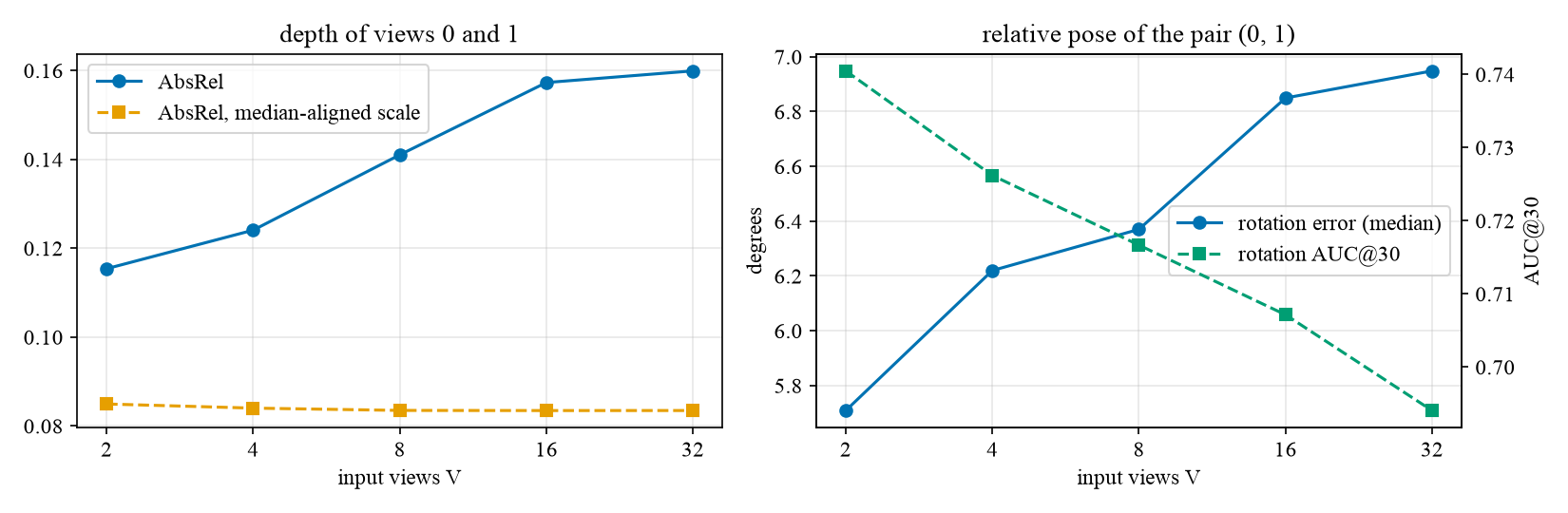
Cost. Runtime and memory grow slowly: 50 ms and 0.69 GiB per scene at V = 2, 59 ms / 0.75 GiB at the training setting V = 8, and 65 ms / 0.98 GiB at V = 32 (batch 1, A100; the timings are single measurements and noisy — V = 24 measured slower than V = 32 — so only the trend is meaningful). At these sizes the fixed cost dominates (16 aggregator blocks, the camera transformer and the DINO encoder launched once per scene); per-frame work is small and global attention over V × 261 tokens is still short (8,352 tokens at V = 32), so the quadratic term has not taken over yet.
Accuracy: fewer views are better for this model, and the controlled table shows why. The standard all-view metrics in (a) get worse with V (validation AbsRel 0.112 → 0.147 → 0.174), but they mix in a changing population of views and pairs. On the two views shared by every V (b), the same trend remains (AbsRel 0.115 → 0.141 → 0.160; rotation error of the pair (0, 1) 5.7° → 6.4° → 6.9°), so it is real, not an averaging artefact. After aligning each scene's depth scale, however, AbsRel is flat (0.0849, 0.0835, 0.0835), while the scale error grows (mean |log ratio| 0.077 → 0.092 → 0.105). The shape of the predicted depth does not depend on V at all, which is consistent with the depth shape coming largely from per-image features, and the whole depth degradation is the global scale.
Why the scale. Targets are normalised so that the centroid of the valid points of all V views lies at distance 1 from camera 0. With V = 2 that scale is a property of the two images the network sees in full; with V = 32 it depends on 30 more views spread over the 32-frame window, and the network has to estimate a quantity it was only trained to estimate for 8 views. Errors in that estimate scale every depth map at once. The pose of a fixed pair degrades more mildly (+1.2° median from V = 2 to 32), as global attention spreads over more frames than in training; translation direction stays poor at every V (median 34–38°, see Q3.2).
Limitations and what would change it. One trained model (V = 8), evaluation only; training with a range of V (as in Q2.3 for Mini-LVSM) or making the scale normalisation independent of V (e.g. reference-view-only scale) would be the natural next experiments.
Anthropic Claude was used to explain course concepts and to polish the writing.