
Yi Zhao (yizhao5). All training and rendering ran on one NVIDIA H100. Every number on this page is read from the metrics files written by the runs; PSNR for the NeRF models is measured on the 100 held-out validation views of each scene.
Pixel coordinates are mapped to [-1, 1] with the first and last pixel at exactly -1/+1, the convention sample_images_at_xy uses (grid_sample with align_corners=True), so a ray and the ground-truth colour it is compared with refer to the same pixel. Each NDC point is lifted to depth 1, unprojected with camera.unproject_points, and the ray direction is the normalised vector from the camera centre to that point.


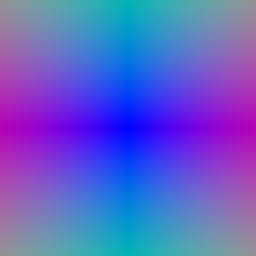
StratifiedRaysampler places n_pts_per_ray depths uniformly between near and far. While training, each depth is jittered uniformly inside its bin (NeRF's stratified sampling), so the network sees every depth over the course of training instead of a fixed grid; at evaluation the bin edges are used so renders are deterministic.


Weights are wi = Ti(1 - exp(-σiΔti)) with Ti = ∏j<i exp(-σjΔtj) computed by a cumulative product (T1 = 1). Colour is ∑ wi ci; depth is the expected termination depth ∑ wi ti, shown normalised by its maximum.
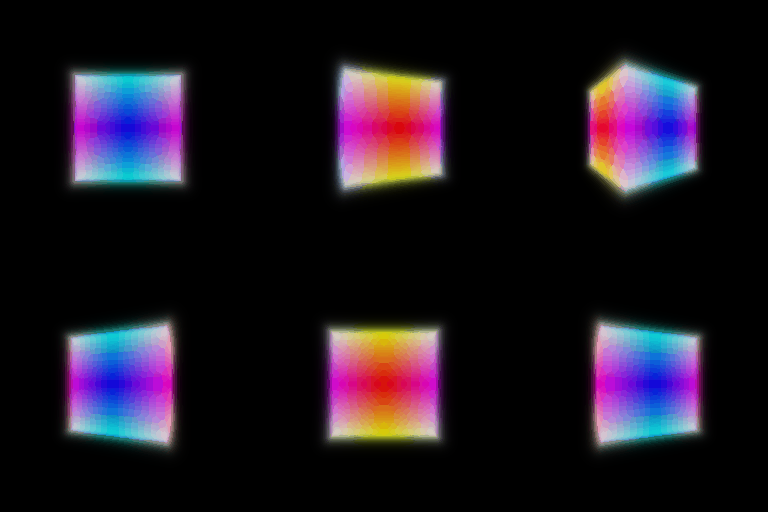


Random rays: a random permutation of all pixel coordinates, first batch_size kept (sampling without replacement). Loss: mean squared error between rendered and ground-truth colours.


Architecture: positional encoding of x (6 frequencies) → 6-layer MLP, 128 units, ReLU, with the encoding re-injected at layer 3 → density head (Linear + ReLU) and colour head (Linear-ReLU-Linear-Sigmoid). Loss: MSE. Settings from nerf_lego.yaml: 250 epochs, 1024 rays per step, 128 samples per ray, 128×128 images.


One thing that had to be fixed first. With PyTorch's default Linear initialisation my first NeRF never trained: the loss stayed flat for 140 epochs. A diagnostic showed the density was exactly zero at every sample from step 0. The default init shrinks the activations at every layer, so after the 6-layer trunk the features are nearly constant and the density takes the sign of its bias; with a negative bias the ReLU outputs 0 everywhere, the render is black, and no gradient reaches the density again. He initialisation for the ReLU layers plus a small positive density bias fixes it (same architecture, same ReLU).
The viewing direction is encoded with 2 harmonic frequencies and concatenated with the 128-d bottleneck features after the density head, so only the colour head sees it (Linear(128+15, 64)-ReLU-Linear-Sigmoid). Density, and therefore geometry, still depends on position alone, as in NeRF. Trained on the materials scene with nerf_materials.yaml (128×128) and nerf_materials_highres.yaml (400×400).
| Materials, validation PSNR (dB) | no view dependence | view dependence | gain |
|---|---|---|---|
| 128 × 128 | 23.80 | 24.57 | +0.77 |
| 400 × 400 | 23.89 | 24.77 | +0.88 |


The materials scene is made of glossy and metallic spheres whose highlights and reflections move with the viewer, which a position-only colour can only average out. Giving the colour head the direction raises the validation PSNR at both resolutions. The visual difference is subtle at this resolution; it is clearest in the highlights on the metallic and glossy spheres in the held-out views below (each panel: prediction | ground truth, 128×128 models of the next table).


To make the trade-off measurable, the same 128×128 setup was trained three times and evaluated on all 100 training views and all 100 held-out views. The third model gives the direction to the trunk as well (view_dependence=early), so even the density can change with the viewpoint.
| Model | train PSNR | validation PSNR | gap |
|---|---|---|---|
| no view dependence | 24.00 | 23.80 | 0.20 |
| direction in the colour head (NeRF) | 24.76 | 24.57 | 0.19 |
| direction in the trunk as well | 25.32 | 24.91 | 0.40 |
Reading the table. Putting the direction into the colour head (NeRF) improves both the training views (24.76 vs 24.00 dB) and the held-out views (24.57 vs 23.80 dB) while the train-validation gap stays the same (0.19 vs 0.20 dB): the extra freedom is spent on real view-dependent appearance, not on memorising pixels. Letting the direction into the trunk too, so that density can also change with the viewpoint, fits the training views best (25.32 dB) and is even a little better on the held-out views here (24.91 dB), but its gap doubles to 0.40 dB. That growing gap is the signature of overfitting.
The trade-off. View dependence lets a model explain what one colour per point cannot (highlights, reflections), but every degree of freedom given to the direction can also explain a training pixel without getting the geometry right. Each surface point is observed from only a handful of directions, and a model whose density depends on the direction no longer has to make the views agree on one 3D shape. On this scene the 100 training cameras surround the object densely and the held-out cameras lie between them, so interpolation still works and the extra capacity is not yet harmful on average; with fewer views or cameras outside the training distribution, the model with the larger gap is the one expected to break first. NeRF's design keeps the benefit and limits the risk: density stays independent of the direction (geometry must be consistent across views), the direction only enters a small late colour head, and it is encoded with few frequencies (2 vs 6 for position), so colour can only vary smoothly with direction.
Two NeRFs of the Q3 architecture. The coarse one is evaluated at 64 stratified samples; its weights (without the two end bins) define a piecewise-constant PDF along each ray, from which 128 more depths are drawn by inverse-CDF sampling (deterministic quantiles at test time). The fine network is evaluated on the union of the 64 + 128 sorted depths. Both networks are trained with the photometric loss; the sampled depths are detached, so the coarse network learns only from its own rendering. Same lego setup as Q3 (250 epochs, 128×128).
| Lego | val PSNR (dB) | train ms / step | render ms / 128² image | parameters |
|---|---|---|---|---|
| Q3: uniform, 128 samples | 25.00 | 7.1 | 26 | 117,764 |
| uniform, 192 samples | 25.34 | 9.3 | 34 | 117,764 |
| coarse 64 + fine 128 | 25.56 | 12.3 | 46 | 235,528 |


Quality. Coarse/fine is the best of the three: +0.56 dB over Q3. Part of that is simply more samples, so the fair comparison is uniform sampling with the same 192 evaluations per ray: coarse/fine is still +0.23 dB ahead, because its 128 extra samples are placed where the coarse weights are large, i.e. around the surface, instead of in empty space.
Speed. A training step costs 1.74× Q3 and 1.31× the equal-sample uniform model, and rendering is slower by a similar factor: the fine pass cannot start until the coarse pass has produced its weights, the two networks double the parameter count, and the coarse samples are evaluated twice (once per network). The gain per sample is real but modest on this small, compact scene at 128×128; it grows when most of the ray is empty space or the resolution is high, where uniform samples are mostly wasted.
Distance network. Positional encoding (6 frequencies) → 6 linear layers of 128 units with Softplus(β=100) activations → 1 signed distance + a 128-d geometry feature. The distance is left unbounded (unlike density it must be able to go negative). Softplus keeps the network smooth, which matters for the Eikonal term (a ReLU network has piecewise-constant gradients). Weights use the geometric initialisation of SAL, so training starts from the SDF of a sphere of radius 1 instead of a random field. Colour network. (geometry feature, encoded position) → Linear-ReLU-Linear-Sigmoid. Eikonal loss: mean of (‖∇d‖ - 1)² at random points in the bounding box, weight 0.02. SDF to density (VolSDF Eq. 2-3): σ(x) = α Ψβ(-d(x)), with Ψβ the CDF of a zero-mean Laplace distribution of scale β.
What α and β do. α is the density deep inside the object (the density at the surface itself is α/2): it sets how opaque the solid is, i.e. how quickly a ray is absorbed once it enters. β sets how wide the transition is: density goes from ~0 to ~α over a band of a few β around the zero level set. Small β is a sharp, almost binary occupancy; large β a soft shell.
1. How does high β bias the learned SDF? Low β? With a high β the density is spread over a thick band around the zero level set, so what the renderer sees is a soft shell rather than the surface. The photometric loss can then be satisfied by a smooth, rounded SDF whose zero set does not have to sit where the true surface is; thin parts and sharp edges are smoothed away or merged (compare the β = 0.3 geometry below, which is visibly rounder and loses the tread and shovel detail). With a low β the density is close to a step at d = 0, so the rendered surface and the zero level set coincide, but only points within a few β of the current surface receive any gradient.
2. Easier to train with low or high β? High β. The density, and hence the loss, varies smoothly over a wide band, so samples far from the current surface still get a gradient and a coarse uniform sampler always has several samples inside the transition. With low β the transition is narrower than the sample spacing (Δt = 0.031 here) and most samples see either ~0 or ~α, which gives sparse, noisy gradients.
3. More accurate surface with high or low β? Low β, provided it can still be trained: VolSDF bounds the opacity error by a term proportional to β, and a sharp transition pins the rendered surface to the zero level set. In my sweep, however, β is not the only knob that matters, which is the more useful observation. At α = 10, lowering β from 0.3 to 0.02 helps (20.95 → 22.41 dB) and then stops helping (22.31 dB at β = 0.01). The limit is α: one sample of fully occupied space absorbs only 1 - exp(-αΔt) = 27% of the light at α = 10, so a ray travels several samples into the object before it is stopped and the rendered surface lies inside the zero set no matter how sharp β is (this is the 'skirt' of half-transparent geometry around the base). At α = 50 a sample absorbs 79%, at α = 100 96%, and every low-β run gains about 1.7-1.9 dB (22.31 → 24.05 → 24.24 dB at β = 0.01). So an accurate surface needs a sharp transition (low β) and a density high enough that the transition is opaque at the sampling resolution (high α).
| α | β | val PSNR (dB) |
|---|---|---|
| 10 | 0.01 | 22.31 |
| 10 | 0.02 | 22.41 |
| 10 | 0.05 | 22.37 |
| 10 | 0.1 | 22.04 |
| 10 | 0.3 | 20.95 |
| 50 | 0.01 | 24.05 |
| 50 | 0.02 | 24.20 |
| 50 | 0.05 | 23.97 |
| 100 | 0.01 | 24.24 |
Best setting: α = 100, β = 0.01 (24.24 dB). All runs use the volsdf_surface.yaml schedule (250 epochs, 128 samples per ray, Eikonal weight 0.02).


The same views for other settings (geometry):


Settings I chose and why. α = 100, β = 0.01 gives the best validation PSNR (24.24 dB) and the cleanest geometry: high α makes the surface opaque within one or two samples, and a β comparable to the sample spacing keeps the transition sharp while still being trainable with 128 uniform samples. The differences among β ≤ 0.05 at a fixed high α are small (within ~0.2 dB), while going from α = 10 to α ≥ 50 is the single largest improvement. Everything else follows volsdf_surface.yaml, with the Softplus distance network and sphere initialisation described above.
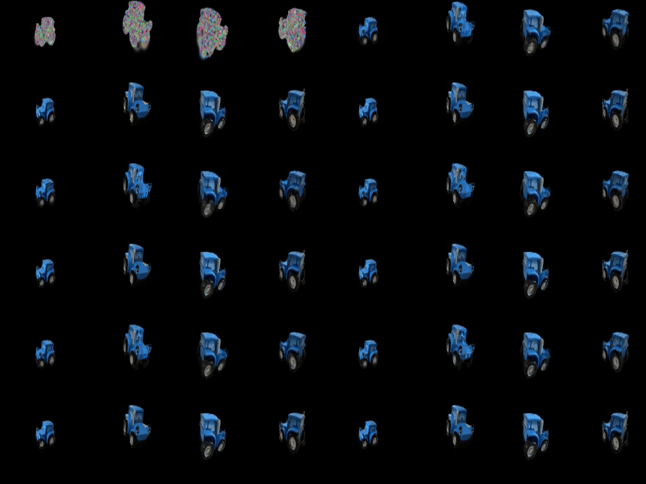
Covariance Σ = R S ST RT (for isotropic gaussians R = I, so Σ = s²I without building a rotation). Projection: Σ' = J W Σ WT JT with the provided Jacobian; 2D means from transform_points_screen. Gaussians are sorted by view-space depth and those behind the camera dropped; α = o·exp(P), Ti = ∏j<i(1-αj) by a cumulative product, and colour, depth and silhouette are ∑ ciαiTi, ∑ ziαiTi and ∑ αiTi. The provided unit tests pass (4/4). Each frame below shows colour, depth and silhouette.
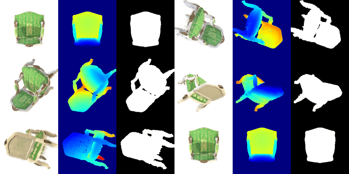
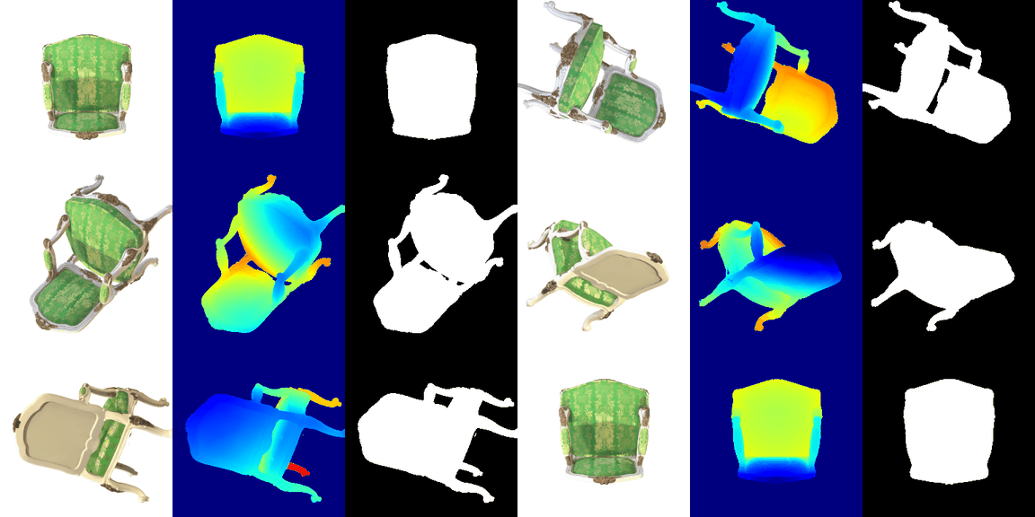
The unit test for compute_cov_2D only passes with W = camera.R. PyTorch3D, however, stores R for row vectors (xcam = xworld R + T), so the column-vector rotation that belongs in Eq. (5) is RT. The two only agree for isotropic gaussians, which is why the difference is easy to miss. For the anisotropic chair the effect is visible: with W = R the ellipses are rotated by the wrong matrix and thin parts turn into fuzzy streaks; with W = RT the legs and the carved frame are crisp. The code keeps the unit-test convention as the default (so the tests pass and the GIF above is the expected output); --transpose_view_rotation switches to RT.


All gaussian attributes are made leaf tensors with gradients (quaternions are not optimised for isotropic gaussians). One Adam optimiser with a separate learning rate per parameter group; loss: L1 between the render and the image. Means live in world units and get the smallest learning rate; log-scales are also kept small because a step in log space changes a gaussian's footprint multiplicatively; colours and opacities can move fast.
| lr means | lr scales | lr colours | lr opacities | iterations | PSNR | SSIM |
|---|---|---|---|---|---|---|
| 0.0005 | 0.005 | 0.02 | 0.05 | 1000 | 29.58 | 0.938 |
| 0.0002 | 0.005 | 0.02 | 0.05 | 1000 | 29.22 | 0.935 |
| 0.001 | 0.005 | 0.05 | 0.05 | 1000 | 29.04 | 0.931 |
| 0.0005 | 0.005 | 0.02 | 0.05 | 3000 | 30.97 | 0.951 |
Lowering the mean learning rate to 0.0002 slows the geometry down (29.22 vs 29.58 dB at 1000 steps); raising the mean and colour rates makes training noisier and ends lower (29.04 dB). With the middle setting, training longer helps the most: 3000 steps reach 30.97 dB / SSIM 0.951, so 1000 steps are not yet converged on this scene. The four runs were compared on the same held-out views that are reported, so the choice among them is itself made on those views; the 3000-step run is the one shown.

colours_from_spherical_harmonics evaluates the real spherical harmonics up to degree 3 (16 coefficients per channel, the same basis and constants as the official 3DGS code) at the unit direction from the camera centre to each gaussian, then adds 0.5 and clamps at 0, the same offset used for the DC-only colours.
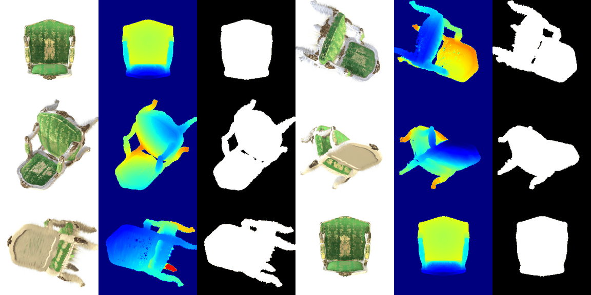

Seen from above, the DC-only render is a flat, uniformly light green. With the full spherical harmonics the backrest and seat are a deeper green, the gold brocade pattern stands out, and the lower part of the backrest is darker than the upper part: the shading now depends on the viewing angle instead of being baked into one average colour.

Looking down onto the seat, the silk shows bright gold sheen on the woven pattern with SH, which is a view-dependent specular effect; the DC colour averages the sheen over all directions and looks washed out and lower in contrast.

From underneath, the two renders are almost identical. The underside is mostly matte wood and fabric seen at a grazing angle, so the higher-order SH terms contribute little; view dependence matters where the material is glossy.
| Setup | iterations | final gaussians | PSNR | SSIM |
|---|---|---|---|---|
| Baseline: Q6 recipe (isotropic, Q6 learning rates, L1), 1000 steps | 1000 | 10,000 | 18.52 | 0.675 |
| Baseline, trained 5000 steps | 5000 | 10,000 | 18.86 | 0.708 |
| Improved (all modifications) | 5000 | 8,569 | 24.78 | 0.900 |
| Improved without densification | 5000 | 10,000 | 23.70 | 0.870 |
| Improved with isotropic gaussians | 5000 | 8,634 | 23.92 | 0.880 |
| Improved with W = R (unit-test convention) | 5000 | 8,624 | 24.39 | 0.889 |

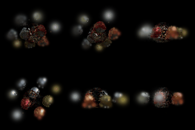


Why the baseline fails. The baseline uses the Q6 setup (isotropic gaussians, the Q6 learning rates, L1 loss) with init_type="random". The reported Q6 truck model was trained for 3000 steps; here the baseline is shown at 1000 steps (18.52 dB) and at 5000 steps (18.86 dB), which bracket that, so it is not just under-trained. Its random init puts all 10,000 isotropic, fully opaque gaussians in a small blob at the centre while the spheres are spread over a much larger area; the gaussians have to travel far, block each other, and many never reach an object, so the renders stay a few blurry blobs.
Modifications in the improved run (relative to Q6; the ablations remove one change at a time from the full recipe, same number of steps):
Each configuration was trained once (one seed), so differences of a few tenths of a dB between ablations should be read as indicative; the gap between the baseline and the improved recipe (6.3 dB) is far larger than that.
Anthropic Claude was used to explain course concepts and to polish the writing.