


Yi Zhao · Andrew ID yizhao5
All models are trained on the single-class (chair) R2N2 split with a frozen-free ResNet-18
encoder trained end to end, and evaluated on the full test split with the F1 score provided in
eval_model.py. Predictions and ground truth are always rendered with the same
camera, lights and shader, so the pictures compare geometry rather than presentation.
Binary cross entropy on logits between the optimised grid and the target occupancy grid. Optimising the grid directly means it leaves [0,1] immediately, so the loss is taken on logits and the isosurface is read from the sigmoid.
Final fitting loss 0.00043 · 30000 iterations, lr 4e-4
Chamfer distance written out with knn_points (squared distances, averaged over points and batch), no pytorch3d.loss helper.
Final fitting loss 0.00019 · 30000 iterations, lr 4e-4, 5000 points
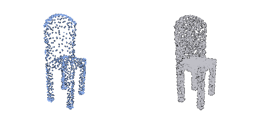


Chamfer on surface samples plus a uniform-weight laplacian smoothing term.
Final fitting loss 0.00032 · 30000 iterations, lr 4e-4, w_smooth 0.1, ico_sphere level 4


F1@0.05 = 70.85
Averaged over all 678 test shapes.


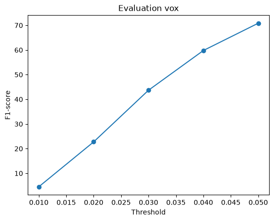
| threshold | precision | recall | F1 |
|---|---|---|---|
| 0.01 | 4.60 | 4.51 | 4.53 |
| 0.02 | 22.94 | 23.14 | 22.73 |
| 0.03 | 43.75 | 45.08 | 43.69 |
| 0.04 | 60.48 | 60.99 | 59.79 |
| 0.05 | 72.67 | 71.10 | 70.85 |
F1@0.05 = 78.89
Averaged over all 678 test shapes.

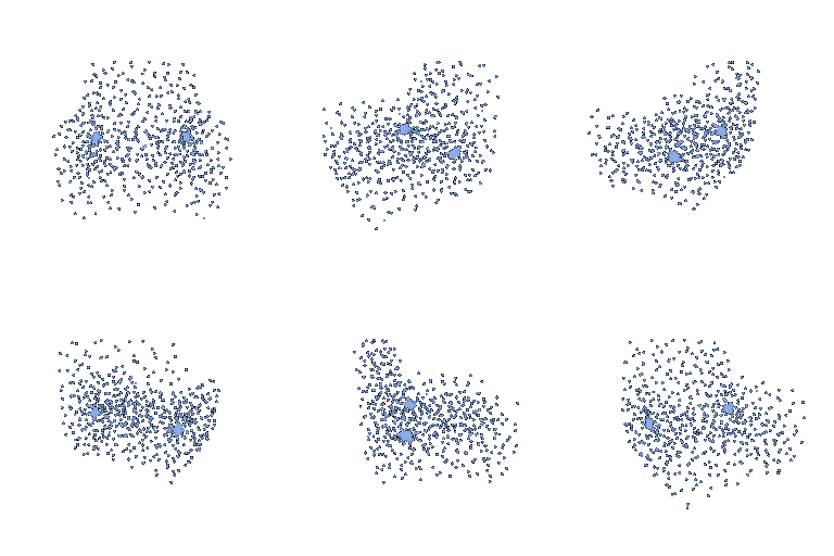


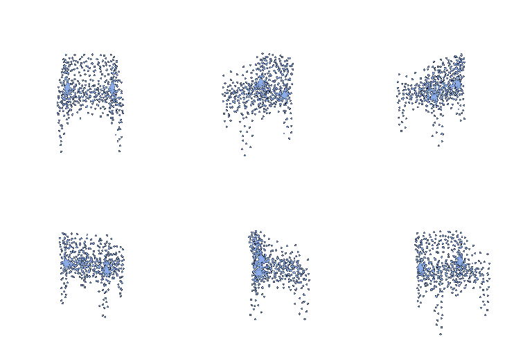

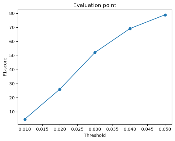
| threshold | precision | recall | F1 |
|---|---|---|---|
| 0.01 | 7.21 | 3.92 | 4.69 |
| 0.02 | 32.93 | 23.26 | 26.03 |
| 0.03 | 56.80 | 50.53 | 52.07 |
| 0.04 | 71.91 | 68.71 | 69.09 |
| 0.05 | 80.84 | 78.74 | 78.89 |
F1@0.05 = 69.49
Averaged over all 678 test shapes.


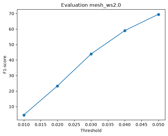
| threshold | precision | recall | F1 |
|---|---|---|---|
| 0.01 | 4.53 | 4.67 | 4.59 |
| 0.02 | 22.38 | 24.64 | 23.31 |
| 0.03 | 42.04 | 46.78 | 43.90 |
| 0.04 | 57.21 | 61.74 | 58.96 |
| 0.05 | 68.36 | 71.41 | 69.49 |
The laplacian weight is 2.0 rather than the default 0.1. At 0.1 the surface folds over itself and stops looking like a chair, even though it scores higher on F1; section 2.4 shows both and explains why the metric prefers the folded mesh. The model reported here is the one a human would call a reconstruction.
| representation | F1@0.05 |
|---|---|
| Voxel grid (Q2.1) | 70.85 |
| Point cloud (Q2.2) | 78.89 |
| Mesh (Q2.3), w_smooth = 2.0 | 69.49 |
Point cloud (Q2.2) scores highest. The ordering follows how directly each representation can place surface samples where the evaluation measures them. The point cloud decoder predicts the evaluated quantity itself -- 3D points -- so nothing is lost between what it optimises (chamfer on those points) and what is scored. The mesh carries the extra constraint of a fixed sphere topology and a smoothness term, which costs accuracy on thin parts and on the gaps between chair legs that a genus-0 surface cannot open. The voxel grid is limited by its 32^3 resolution: a leg thinner than one voxel either disappears or becomes a blocky column, and the marching-cubes surface is then sampled to produce the points that get scored.
The mesh model is retrained with the laplacian weight w_smooth set to each of
the values below, everything else fixed (30000 iterations, batch 32, lr 4e-4, ico-sphere level 4).
| w_smooth | F1@0.05 |
|---|---|
| 0.0 | 75.77 |
| 0.1 | 72.97 |
| 0.5 | 73.24 |
| 2.0 | 69.49 |


F1@0.05 across the sweep: w=0.0 gives 75.8, w=0.1 gives 73.0, w=0.5 gives 73.2, w=2.0 gives 69.5. The ends are what matter: the unsmoothed mesh (w=0.0) scores 75.8 and the most smoothed one (w=2.0) scores 69.5, a gap of 6.3 points, while the two middle settings are separated by less than the evaluation noise. The interesting part is that this is the opposite of what the renders say.
The laplacian term pulls every vertex towards the centroid of its neighbours, which shrinks thin
structure (chair legs, arm rails) and rounds off the concave joint between seat and back; both
move surface samples away from the ground truth and cost F1 directly. What the term buys is
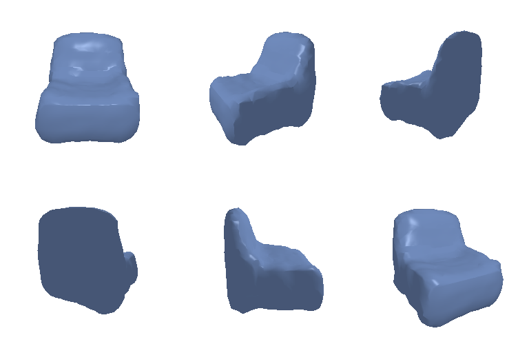
regularity, not accuracy: at w_smooth = 0 the mesh is visibly crumpled, with
spikes and self-crossings, but F1 scores points sampled on the surface, and a spike displaces
only the handful of samples that land on it, so the metric hardly notices. At
w_smooth = 2.0 the surface is clean and the chair is unmistakable, and the score is
the worst of the four.
So on this task F1@0.05 is not a proxy for mesh quality: the best-scoring setting produces the worst-looking mesh. Which setting to ship depends on what the mesh is for. If it feeds a metric like this one, take the small weight; if a human or a downstream geometric operation sees it, the regularity is worth the points. The renders above are the same test object in each column, but the input view is drawn at random per epoch by the dataset, so the photographs differ between columns.
The two end points are real test images; every shape between them is decoded from a linear interpolation of their ResNet-18 features. The chair back and the legs deform continuously rather than snapping between memorised shapes, which is what a learned shape space -- as opposed to a lookup table -- looks like.

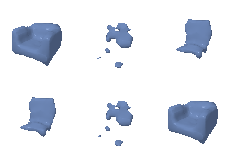
2477 of the 32768 voxels come out above p = 0.8 and 28152 below p = 0.2, leaving only 2139 (6.5%) in the uncertain band between. The occupancy field the network produces is sharp: the three panels at 0.2, 0.5 and 0.8 enclose almost the same solid, which is what a well-separated field looks like. This was not true of the first, under-trained model, where 0 voxels reached 0.8 and the 0.8 panel was blank (vox_confidence_320k.txt, kept next to this page); the next probe follows that thread, because an unconfident field and a fixed 0.5 level set interact badly.

| voxels | count |
|---|---|
| voxels with p > 0.8 (confident occupied) | 2477 |
| voxels with p < 0.2 (confident empty) | 28152 |
| voxels in between (uncertain) | 2139 |
| total voxels | 32768 |
When the field is not yet sharp, the 0.5 level set cuts through a soft shell, and on some shapes it encloses nothing at all. On the first, under-trained voxel model (a third of the training budget) that is exactly what happened: 49 of the 678 test shapes came out empty at the default threshold and were scored F1 = 0.
| isovalue | F1@0.05 | empty predictions |
|---|---|---|
| 0.2 | 58.40 | 0 / 678 |
| 0.3 | 67.05 | 2 / 678 |
| 0.4 | 64.16 | 15 / 678 |
| 0.5 | 53.96 | 49 / 678 |
| isovalue | F1@0.05 | empty predictions |
|---|---|---|
| 0.2 | 61.56 | 0 / 678 |
| 0.3 | 68.89 | 0 / 678 |
| 0.4 | 71.26 | 1 / 678 |
| 0.5 | 70.09 | 1 / 678 |
On the under-trained model the threshold was worth 13.1 points (54.0 at 0.5 against 67.1 at 0.3). On the reported model the same sweep is nearly flat: 70.1 at the default against a best of 71.3 at 0.4, and 1 shape comes out empty. So the miscalibration was a symptom of under-training rather than a property of the loss: a network that has not yet learned to be confident hedges, and hedging interacts badly with a fixed level set. Everything reported above uses the unmodified 0.5.
For 100% of the test images the closest of the 200 sampled training chairs is nearer to the prediction than the chair the prediction was asked to reconstruct (mean chamfer 0.0616 against 0.1128). The point-cloud model, which scores far better, is also the one that does this less often (68%) -- the probe tracks how instance-specific a reconstruction is, and it ranks the two decoders the same way F1 does. The reading is not that the network stores a lookup table, which the interpolation above rules out, but that it outputs a plausible chair conditioned on the image, and the better the model the closer that plausible chair sits to the particular one it was shown.
| quantity | value |
|---|---|
| mean chamfer(prediction, its own ground truth) | 0.11279 |
| mean chamfer(prediction, nearest TRAINING shape) | 0.06161 |
| fraction where a training shape is closer than GT | 1.00000 |
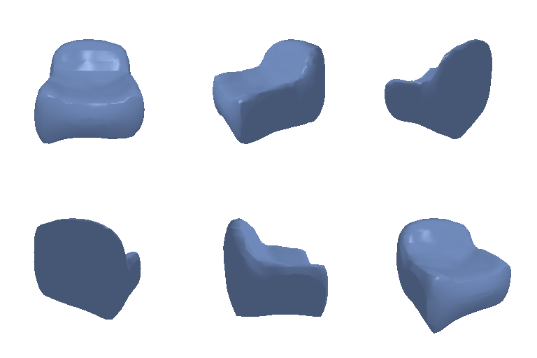
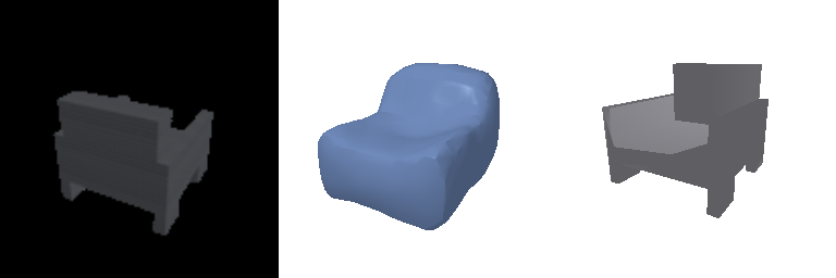
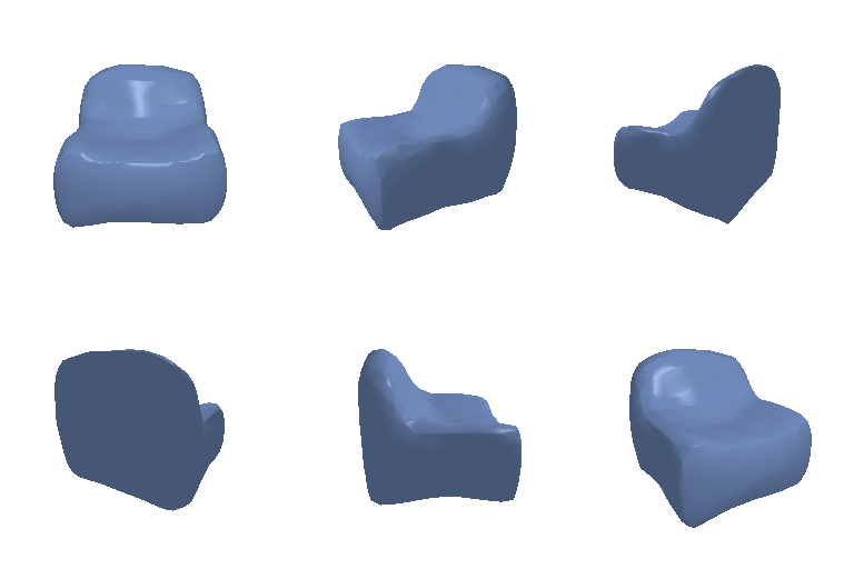
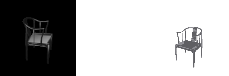
Two of the three options are implemented: an implicit occupancy decoder (3.1) and a parametric surface decoder (3.2). The implicit decoder is shown in three variants, because the first one scored far below the convolutional decoder and a single number could not say why:
F1@0.05 = 34.19
Averaged over all 678 test shapes.
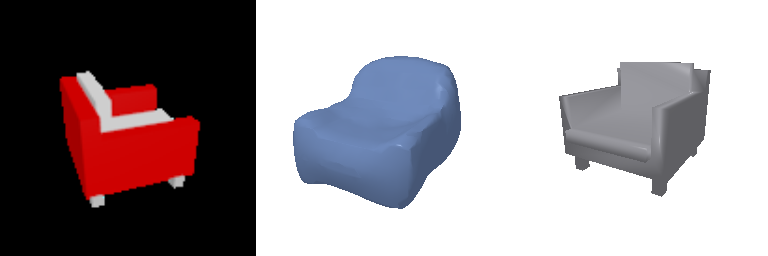

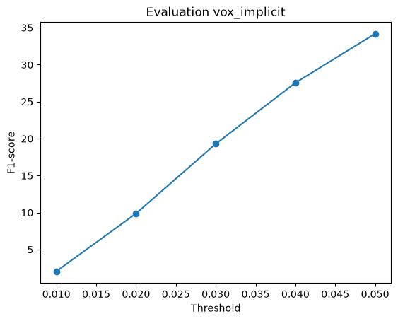
| threshold | precision | recall | F1 |
|---|---|---|---|
| 0.01 | 2.68 | 1.90 | 2.06 |
| 0.02 | 14.22 | 8.65 | 9.87 |
| 0.03 | 28.66 | 16.59 | 19.29 |
| 0.04 | 40.53 | 23.66 | 27.55 |
| 0.05 | 49.24 | 29.45 | 34.19 |
Against the Q2 decoder for the same representation: -36.66 F1@0.05.
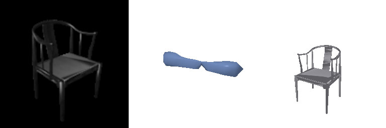
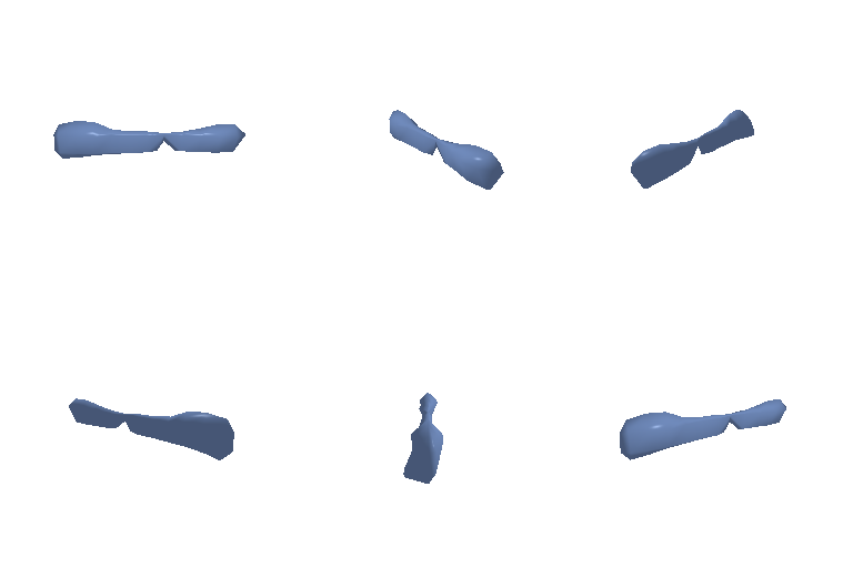
F1@0.05 = 34.36
Averaged over all 678 test shapes.
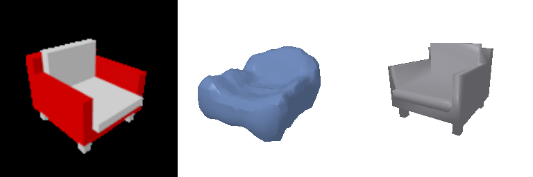
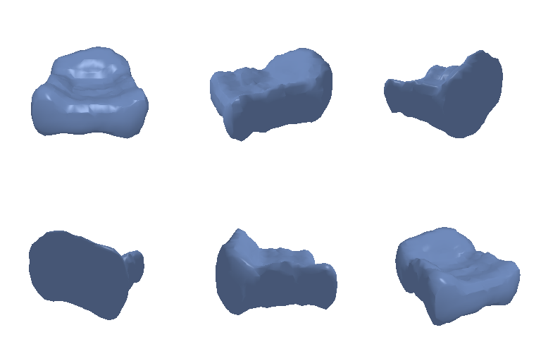
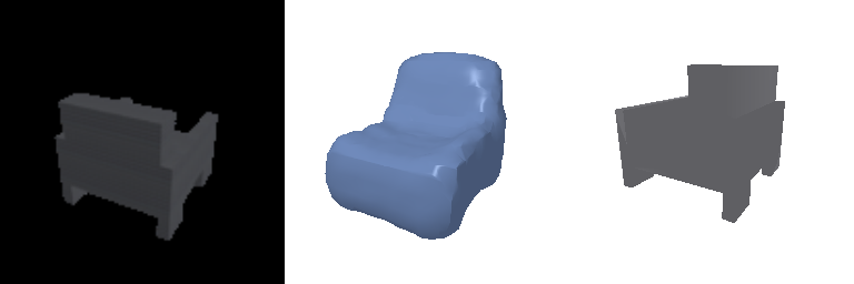
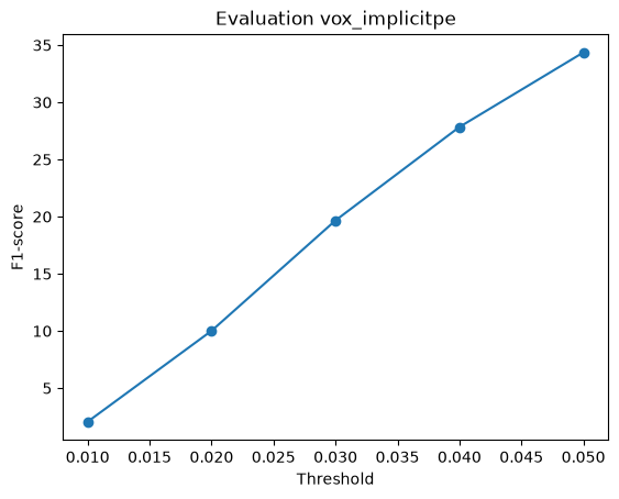
| threshold | precision | recall | F1 |
|---|---|---|---|
| 0.01 | 2.59 | 1.91 | 2.06 |
| 0.02 | 14.35 | 8.91 | 10.02 |
| 0.03 | 28.99 | 17.11 | 19.67 |
| 0.04 | 40.64 | 24.08 | 27.84 |
| 0.05 | 49.49 | 29.74 | 34.36 |
Against the Q2 decoder for the same representation: -36.49 F1@0.05.
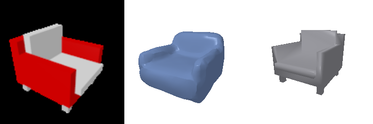
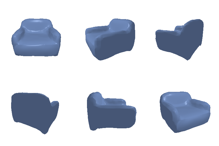
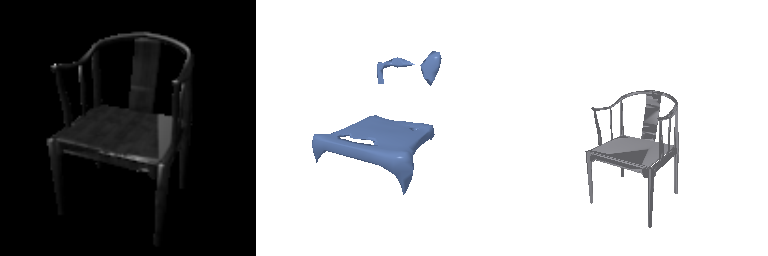
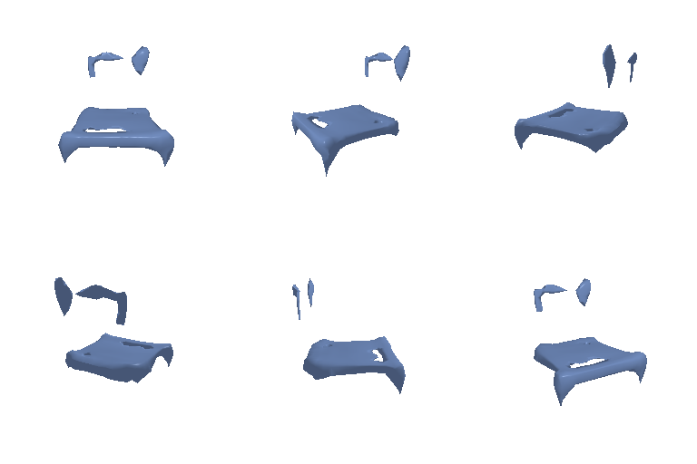
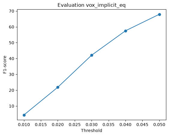
F1@0.05 = 67.92
Averaged over all 678 test shapes.
| threshold | precision | recall | F1 |
|---|---|---|---|
| 0.01 | 4.54 | 4.31 | 4.35 |
| 0.02 | 22.74 | 22.04 | 21.84 |
| 0.03 | 43.67 | 42.89 | 42.08 |
| 0.04 | 60.01 | 58.18 | 57.49 |
| 0.05 | 71.69 | 67.76 | 67.92 |
Against the Q2 decoder for the same representation: -2.93 F1@0.05.
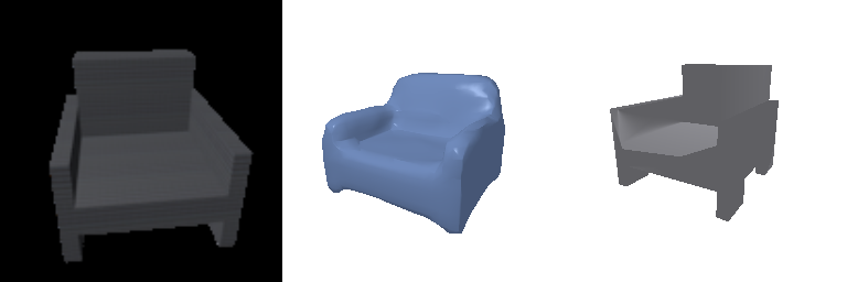
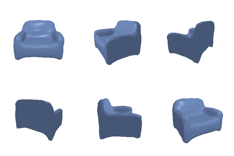
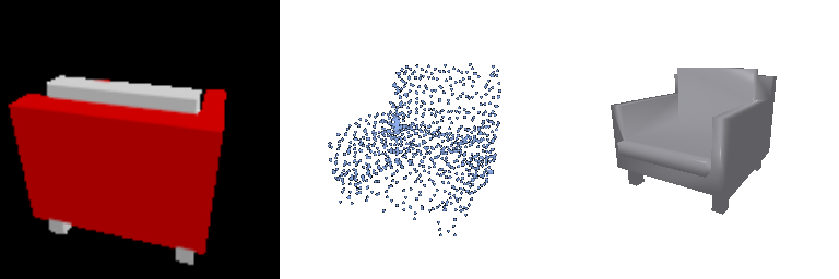
F1@0.05 = 75.44
Averaged over all 678 test shapes.
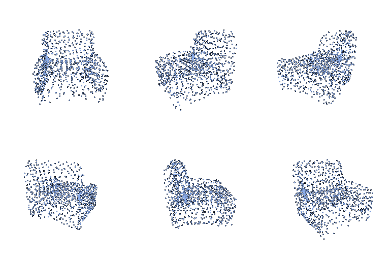

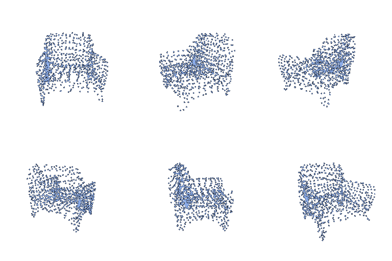

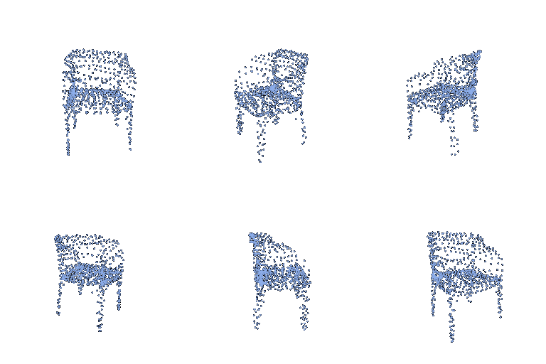
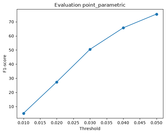
| threshold | precision | recall | F1 |
|---|---|---|---|
| 0.01 | 5.84 | 5.01 | 5.23 |
| 0.02 | 28.42 | 27.33 | 27.42 |
| 0.03 | 50.59 | 51.50 | 50.48 |
| 0.04 | 65.82 | 66.62 | 65.71 |
| 0.05 | 75.90 | 75.79 | 75.44 |
Against the Q2 decoder for the same representation: -3.46 F1@0.05.
The equal-budget control settles it, and not the way the first two runs suggested: at a matched 960k samples the implicit decoder lands within about three points of the convolutional one, against a gap of roughly thirty-five when it was starved. Almost all of what looked like an architectural deficit was training budget. This is worth stating plainly because the earlier reading was wrong: at batch 8 the implicit decoder's training loss appeared to plateau around iteration 4000, which I took as a capacity limit; run at batch 16 for long enough it keeps improving and closes nearly the whole gap. A flat loss curve on a small batch is not evidence of saturation.
The Fourier features are the other negative result. Lifting the coordinate to 6 octaves of sin/cos, the standard remedy for an MLP's low-frequency bias, changed nothing at the small budget (34.4 against 34.2). Whatever limits this decoder, it is not the frequency content of the coordinate encoding.
--load_feat was not used: the ResNet-18 encoder runs on the images.