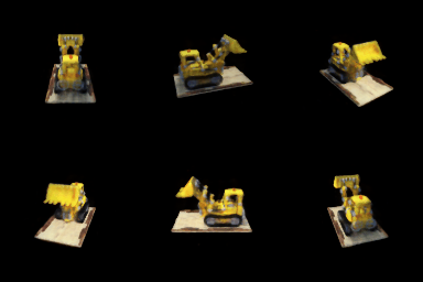
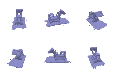
A. Neural Volume Rendering (60 points)
1. Differentiable Volume Rendering
1.1. Familiarize yourself with the code structure
The pipeline connects camera rays, point sampling, an implicit scene, and volume rendering.
1.2. Outline of tasks
I implement ray sampling, point sampling, and compositing to render an implicit scene.
1.3. Ray sampling (5 points)
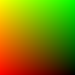
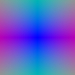
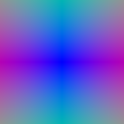
Camera rays map image pixels to viewing directions in world space.

1.4. Point sampling (5 points)
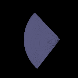
Uniform samples along each ray provide the points used for volume rendering.

1.5. Volume rendering (20 points)
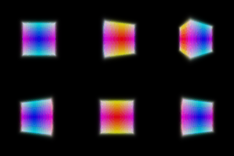
Volume rendering combines sampled colors and densities into color and normalized depth images.


2. Optimizing a Basic Implicit Volume
2.1. Random ray sampling (5 points)
Random pixel samples provide batches of camera rays for training.
2.2. Loss and training (5 points)
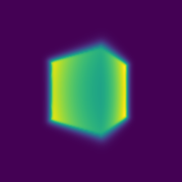
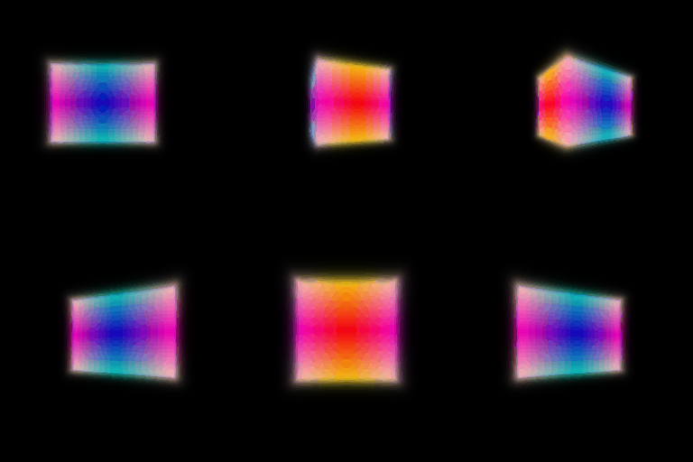
Minimizing color mean squared error (MSE) recovers the box center (0.25, 0.25, 0.00) and side lengths (2.01, 1.50, 1.50).
2.3. Visualization
The optimized box reaches a training-view peak signal-to-noise ratio (PSNR) of 61.27 dB and structural similarity (SSIM) of 0.99998.

3. Optimizing a Neural Radiance Field (NeRF) (20 points)
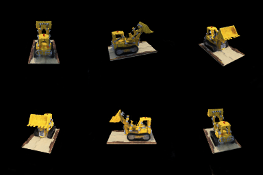
A 6-layer, 128-unit multilayer perceptron (MLP) with positional encoding learns the Lego scene for novel-view rendering.
| Model | PSNR (dB) | SSIM |
|---|---|---|
| Lego NeRF | 25.57 | 0.9000 |

4. NeRF Extras (choose one; more than one is extra credit)
4.1. View Dependence (10 bonus points)
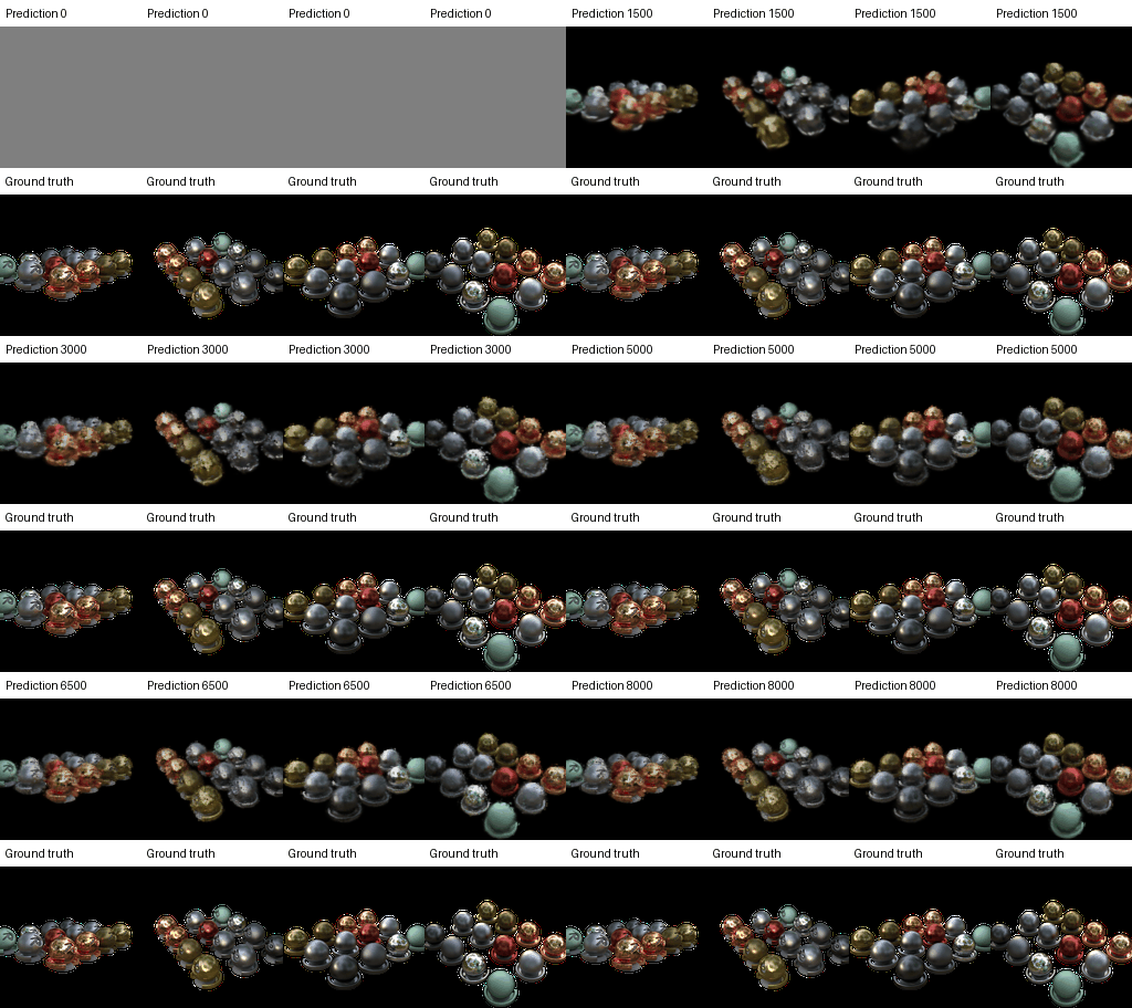
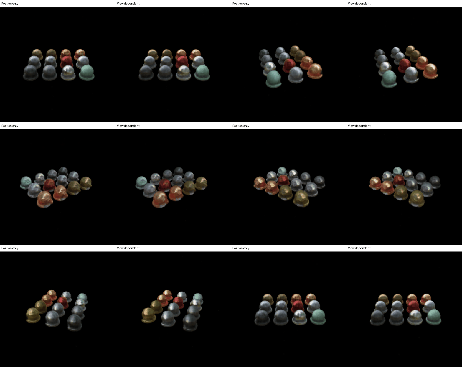
View-dependent color changes with camera direction, allowing it to capture reflections that position-only color cannot, though this flexibility can also overfit; with matched training on 100 materials images at 400 x 400, view dependence changes held-out PSNR by +1.06 dB.
| Model | PSNR (dB) | SSIM |
|---|---|---|
| Position only | 24.27 | 0.8408 |
| View dependent | 25.33 | 0.8561 |

4.2. Coarse/Fine Sampling (10 bonus points)
Coarse/fine sampling combines 64 uniform and 128 importance samples per ray, compared with 192 uniform samples.
| Model | PSNR (dB) | SSIM |
|---|---|---|
| Uniform | 26.11 | 0.9179 |
| Coarse and fine | 26.11 | 0.9185 |
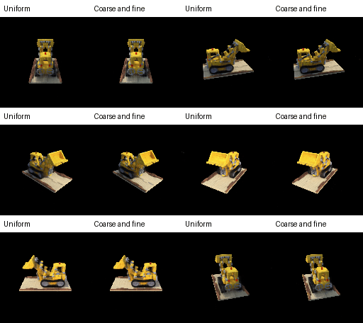
Coarse/fine sampling makes the red rear lights and roof-mounted warning beacon easier to distinguish, with a more vivid red color.
This small quality gain costs more computation: the coarse network evaluates 64 samples and the fine network evaluates all 192 merged samples, versus 192 evaluations for uniform sampling; the second network also increases memory use.
4.3. Volume Rendering with Signed Distance Functions: VolSDF (10 bonus points)
A neural signed distance function (SDF) defines the surface through VolSDF density, with alpha=80 and beta=0.01 selected by validation PSNR among the seven tested settings.
Alpha scales density, making the interior more opaque as it increases, while beta controls the width of the density transition around the surface; the selected small beta favors sharper boundaries, and alpha=80 gave the best validation result.
| Alpha | Beta | Validation PSNR (dB, 4 views) | Test PSNR (dB, 200 views) | Test SSIM |
|---|---|---|---|---|
| 10 | 0.05 | 21.93 | 21.69 | 0.7787 |
| 10 | 0.1 | 21.43 | 21.15 | 0.7583 |
| 40 | 0.05 | 22.71 | 22.62 | 0.8104 |
| 40 | 0.02 | 22.91 | 22.83 | 0.8219 |
| 120 | 0.5 | 13.67 | 12.62 | 0.3824 |
| 120 | 0.01 | 22.82 | 22.81 | 0.8291 |
| 80 | 0.01 | 22.97 | 22.96 | 0.8368 |
| Question | Interpretation |
|---|---|
| How does beta bias the learned SDF? | High beta spreads density across a wider region around the zero level set, allowing blurred boundaries and loss of fine geometric detail; low beta concentrates the transition near the zero level set, favoring sharper surfaces. |
| Is training easier with high or low beta, and why? | A moderately high beta is generally easier to train because more samples along each ray receive useful gradients; low beta confines these gradients to a narrow region that coarse sampling can miss. |
| Which is more likely to recover an accurate surface, and why? | Low beta generally favors more accurate geometry because the rendered density boundary lies closer to the SDF zero level set, reducing surface blurring; this requires sufficient sampling and successful optimization, so smaller beta is not always better in practice. |