Assignment 3: Neural Volume Rendering
1. Differentiable Volume Rendering
1.3 Ray sampling
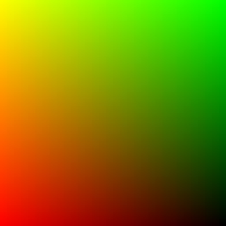
vis_grid)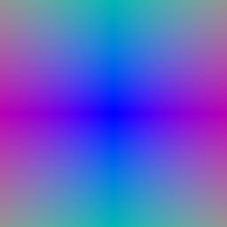
vis_rays)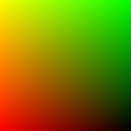
ta_images/grid.png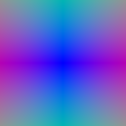
ta_images/rays.pngCamera 0 of the spiral, 256×256.
1.4 Point sampling
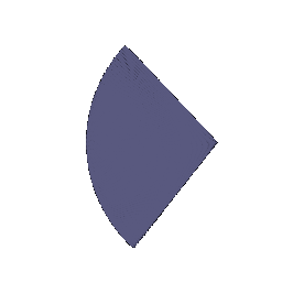
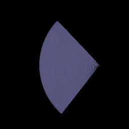
ta_images/sample_points.png)Sample points of camera 0's rays, drawn with render_points. To fit
on a 4 GB GPU, only every 4th row and column of rays is drawn (4,096 rays × 64 points).
1.5 Volume rendering
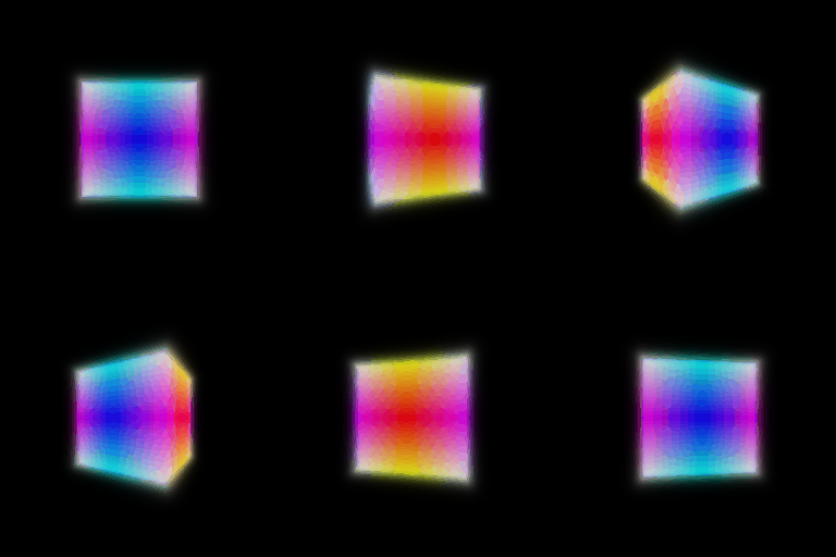
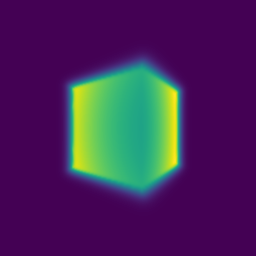
The depth map uses the spiral camera 36° in, which is the README's camera 2 of 20 (camera 6 of my 60).
Extra: a rounded box SDF
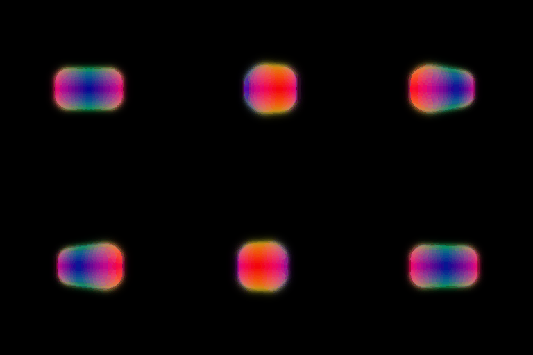
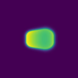
I added RoundBoxSDF to sdf_dict (config
configs/roundbox.yaml): a 2.0 × 1.2 × 1.2 box with corner radius 0.4.
It is the box SDF with the half sizes reduced by the radius, minus the radius:
q = |p − c| − (s/2 − r) d(p) = ‖max(q, 0)‖ + min(maxk qk, 0) − r
2. Optimizing a basic implicit volume
| Parameter | x | y | z |
|---|---|---|---|
| Box center | 0.25 | 0.25 | 0.00 |
| Box side lengths | 2.01 | 1.50 | 1.50 |
Rounded to 2 decimals. Final MSE on the last batch: 1.1 × 10⁻⁶.
Visualization






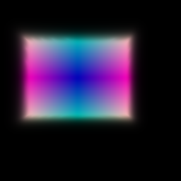



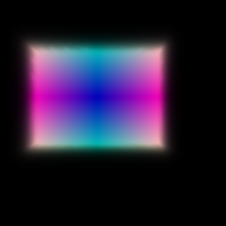

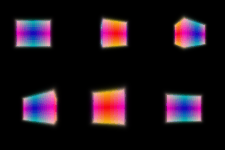
The optimized box matches the ground truth in all four views. Starting from a cube at the origin, it moved +0.25 along x and y and stretched to 2.0 units along x, which is the long side seen in views 2 and 3.
3. Optimizing a Neural Radiance Field (NeRF)
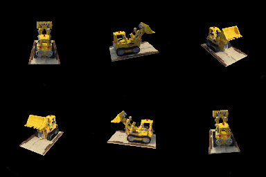
val PSNR 24.25 dB
Training took 48 ms per step, about 20 minutes for 25,000 steps. The bulldozer's arm, bucket and treads are recovered; thin parts such as the bucket's hydraulic lines stay blurry at 128×128.
4. NeRF extras
4.1 View dependence
val PSNR 22.93 dB

val PSNR 23.51 dB
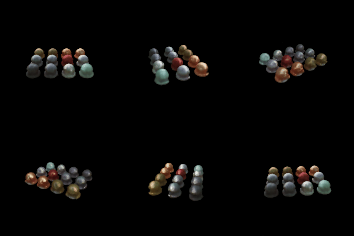
val PSNR 23.65 dB
Same frames, cropped

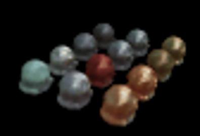


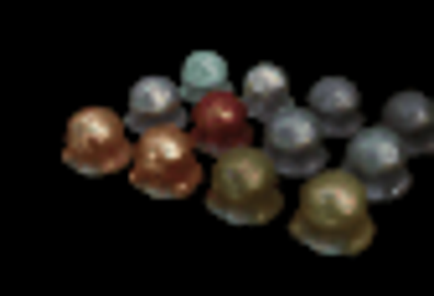

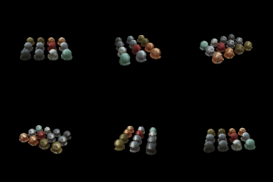
- Without view dependence, each point must have one color for every view. The glossy and metallic balls show highlights that move with the camera, so the network averages them into a noisy, speckled texture painted onto the surface.
- With view dependence, the balls look smooth, and the highlights are coherent blobs that belong to each ball's material. Validation PSNR rises by 0.58 dB. The cost is small: 47 ms vs. 43 ms per step.
- At 400×400, the same network resolves the sharp reflections on the metal balls. Each step still uses 1,024 rays, so training cost stays the same; only rendering 60 frames is slower.
Trade-off between view dependence and generalization
Given enough freedom, a view-dependent color can explain each training image by itself instead of agreeing on one geometry. This is the shape-radiance ambiguity: a wrong surface with the right per-view colors fits the training views but fails on new ones. My model limits this in three ways. Density cannot see the direction. The direction uses only 2 harmonics, so color can vary only smoothly with the viewpoint. And the direction joins the network only after the bottleneck. With 100 training views, the extra freedom improved held-out views here. With fewer views or more direction frequencies, I would expect it to start overfitting: floaters near the cameras, and highlights that pop on validation views.
4.2 Coarse/fine sampling
val PSNR 24.25 dB

val PSNR 24.98 dB
| Network evaluations per ray | ms per step | val PSNR (dB) | |
|---|---|---|---|
| Q3, one network | 128 | 48 | 24.25 |
| Coarse + fine | 64 + 192 | 83 | 24.98 |
Importance sampling places most fine samples on the surface instead of in empty space. That sharpens the treads, the arm joints and the edges of the base, and it adds 0.74 dB. The price is two networks and twice the network evaluations per ray, which made each step 1.7× slower. This comparison does not hold compute fixed. A single network with 256 stratified samples would be the fairer speed-matched baseline, but I did not run it.
4.3 VolSDF
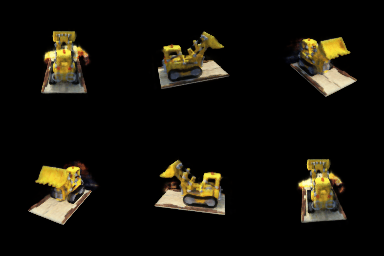
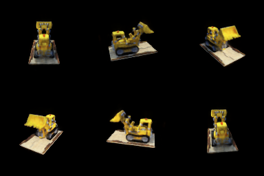
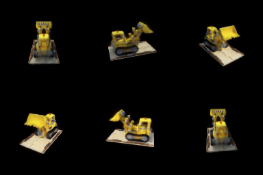
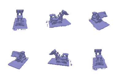
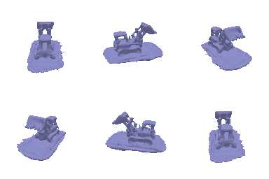
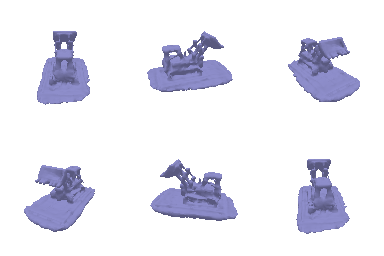
Geometry is the zero level set extracted by marching cubes at 128³. All runs use α = 10, eikonal weight 0.02, lr 5e-4 and 250 epochs on lego at 128×128.
Why the initialization mattered
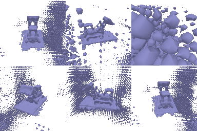
val PSNR 22.38 dB
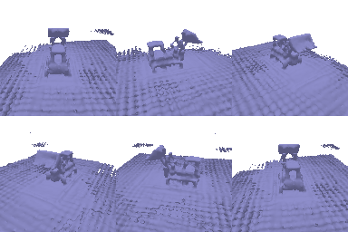
val PSNR 21.83 dB
What α and β do
α is the density deep inside the object: σ tends to α as d tends to −∞, and on the surface (d = 0) σ = α/2. A larger α makes the interior more opaque. β is the width of the transition. Density falls from α to 0 over a band a few β thick around the zero level set, and as β → 0, σ becomes a step function: α inside, 0 outside.
- How does high β bias the learned SDF, and low β? With high β, density leaks over a thick band on both sides of the surface. The renders can then be matched by a blurry shell, and the zero level set does not have to sit where the visible surface is. It tends to drift and inflate, like the thicker base at β = 0.1. With low β, density is concentrated at d = 0. The only way to render the right image is to put the zero level set exactly on the surface, so the SDF is pushed toward a sharp, accurate surface.
- Is an SDF easier to train with low or high β? High β. The density, and so the rendering loss, varies smoothly with d over a wide band. Samples far from the current surface still get gradient, and a stratified sampler with 128 samples always hits that band. With low β, density is nearly flat away from the surface, so gradients vanish. Training also becomes sensitive to whether any sample falls in the thin band; it is the less stable setting (the ReLU run at β = 0.02 broke apart).
- Is an accurate surface more likely with high or low β? Low β, for the reason in question 1: density concentrated at the zero level set ties the SDF's surface to the rendered surface. It needs good initialization and enough samples near the surface to train. Here β = 0.02 gave the sharpest edges, on the arm and the cab, but also small fragments near the base. β = 0.1 was the smoothest and most bloated.
Chosen settings. β = 0.05 gave the best balance: a clean, complete mesh with no fragments, sharper than β = 0.1, and the highest PSNR (22.39 dB). The sphere initialization with softplus mattered far more than β. I kept α = 10 and the eikonal weight 0.02 from the starter config.
5. 3D Gaussian rasterization
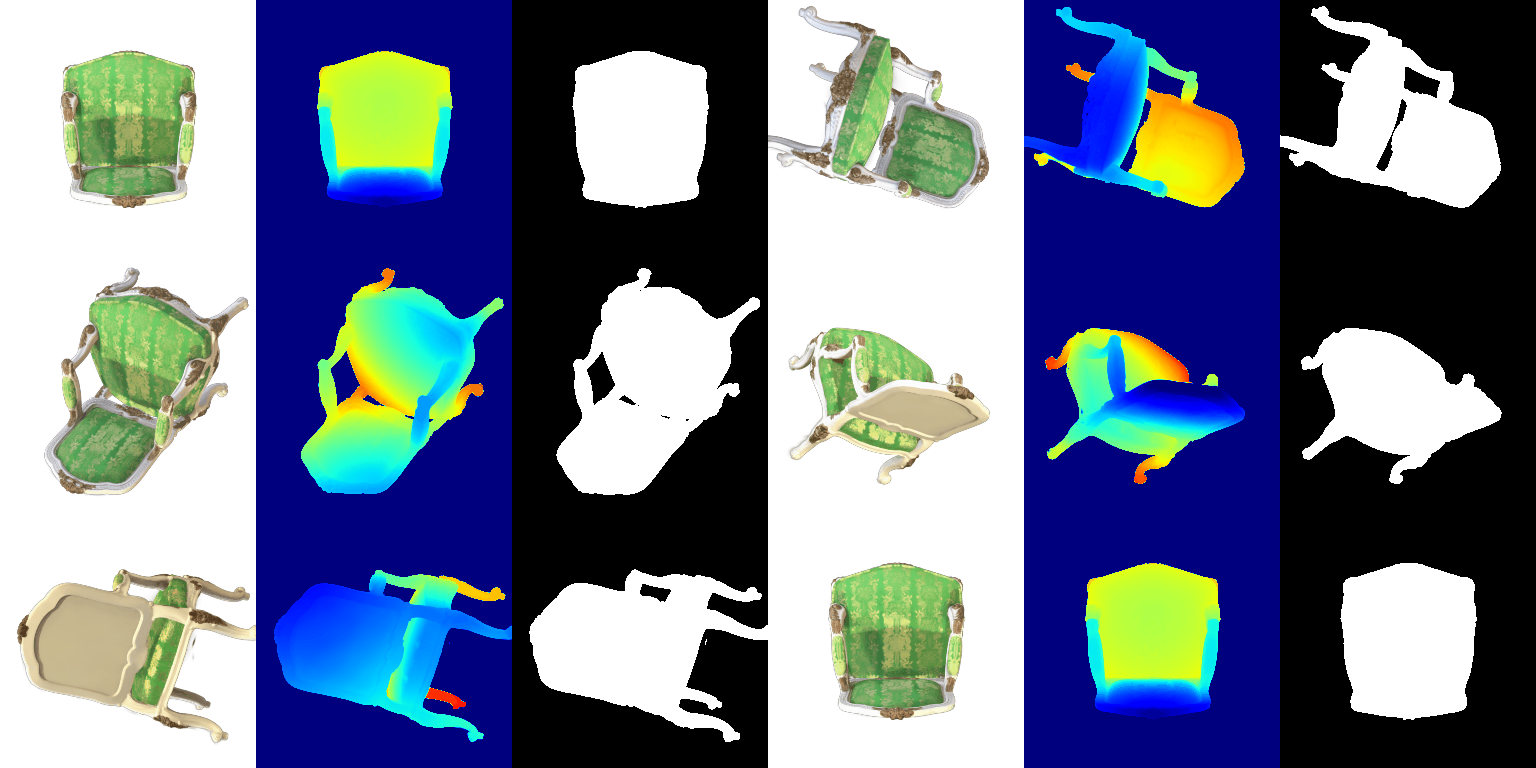
283,873 anisotropic Gaussians, DC colour only. 60 views at 15 fps, along the starter's camera path, which changes azimuth and elevation together.
The world-to-view rotation W, and the unit tests
PyTorch3D multiplies row vectors (xview = xworld R + T), so the rotation acting on column vectors is W = RT. The unit tests' expected covariances were computed with W = R instead. Rendering the chair both ways shows which is right:
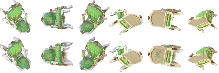
The code uses W = RT, which passes tests 1 and 3. Setting
GS_W_CONVENTION=R switches to the tests' convention, and then all 4 tests pass.
6. Training 3D Gaussian representations

| Parameter | Learning rate |
|---|---|
| Means | 0.0005 |
| Scales (log) | 0.005 |
| Colours | 0.02 |
| Opacities (pre-sigmoid) | 0.01 |
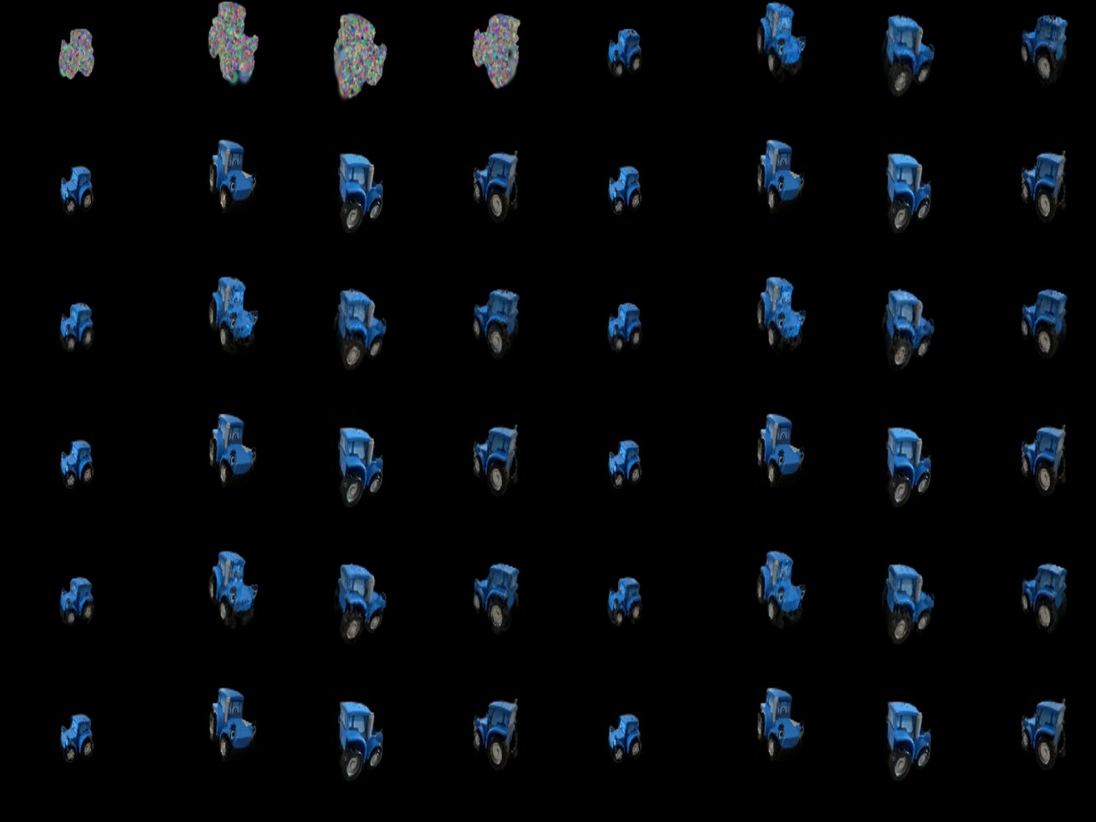
1,000 iterations of Adam with an L1 loss, one training view per step, isotropic Gaussians initialized from the 10,000 provided points. Held-out views: PSNR 29.72 dB, SSIM 0.940. The means get the smallest step, since the point cloud already puts them on the surface; opacities and colours get the largest. Training took about 10 minutes, at 2,048 Gaussians per splat.
7. Extensions
7.1 Rendering using spherical harmonics

Same frames, side by side
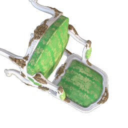
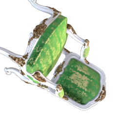
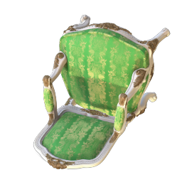
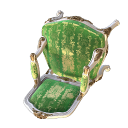
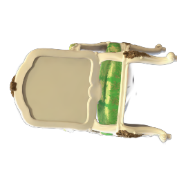
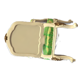
- Frame 10 (looking into the seat): with DC only, the cushions are a flat, bright green. With spherical harmonics, the green is deeper and varies across the seat, and the gold embroidery stands out with highlights, so the fabric looks like satin instead of paint.
- Frame 25 (front of the backrest): the same difference. The DC backrest is evenly bright, while the spherical-harmonics backrest is darker toward its edges and the pattern has more contrast.
- Frame 45 (underside): the two are almost identical. The plain wooden board is close to diffuse, so its colour hardly depends on the view, and the DC term already captures it.
7.2 Training on a harder scene
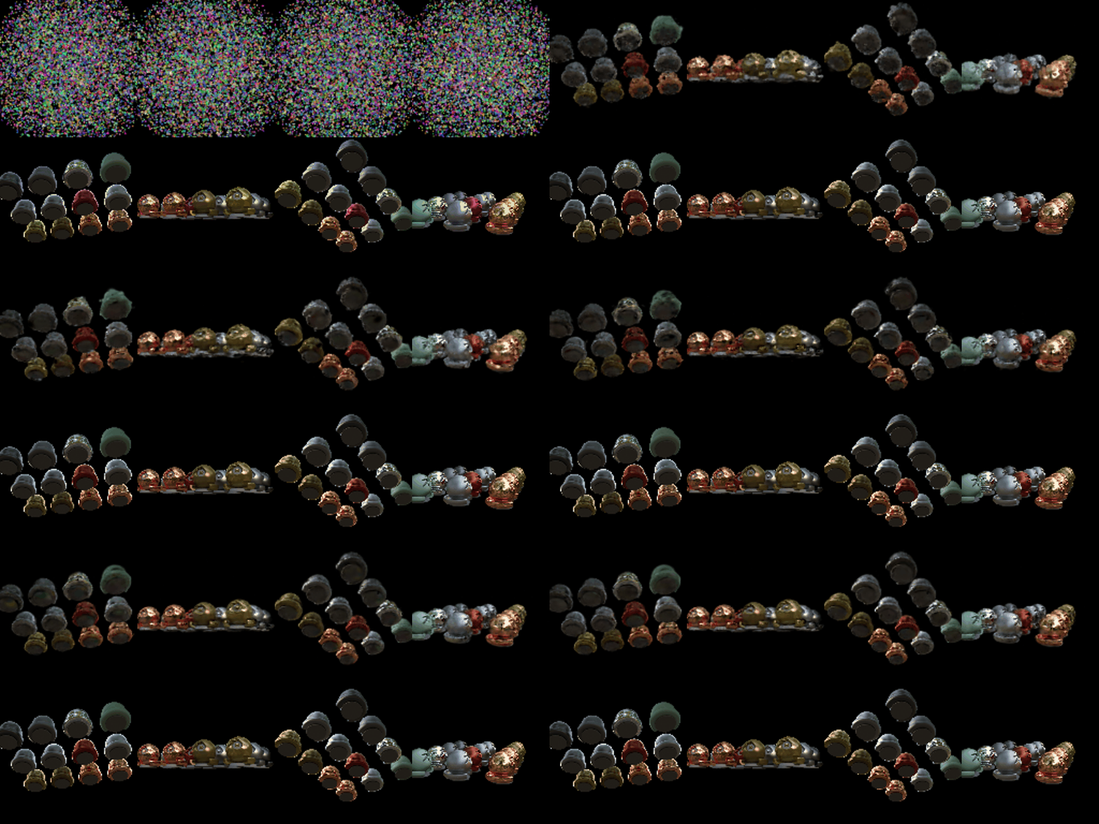
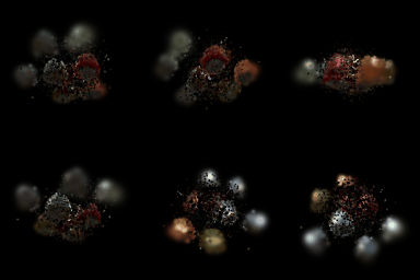
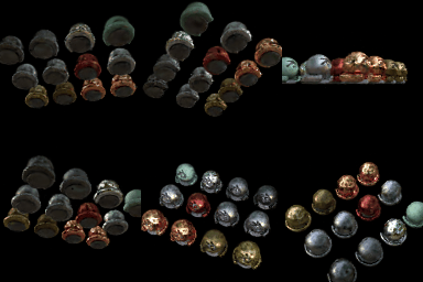
The materials scene at 128×128 from 10,000 random points (100 training views, held-out PSNR and SSIM on the 100 validation views).
| Iterations | Gaussians at the end | PSNR (dB) | SSIM | |
|---|---|---|---|---|
| Baseline (Q6 setup) | 1,000 | 10,000 | 17.53 | 0.655 |
| Improved | 3,000 | 22,137 | 23.98 | 0.887 |
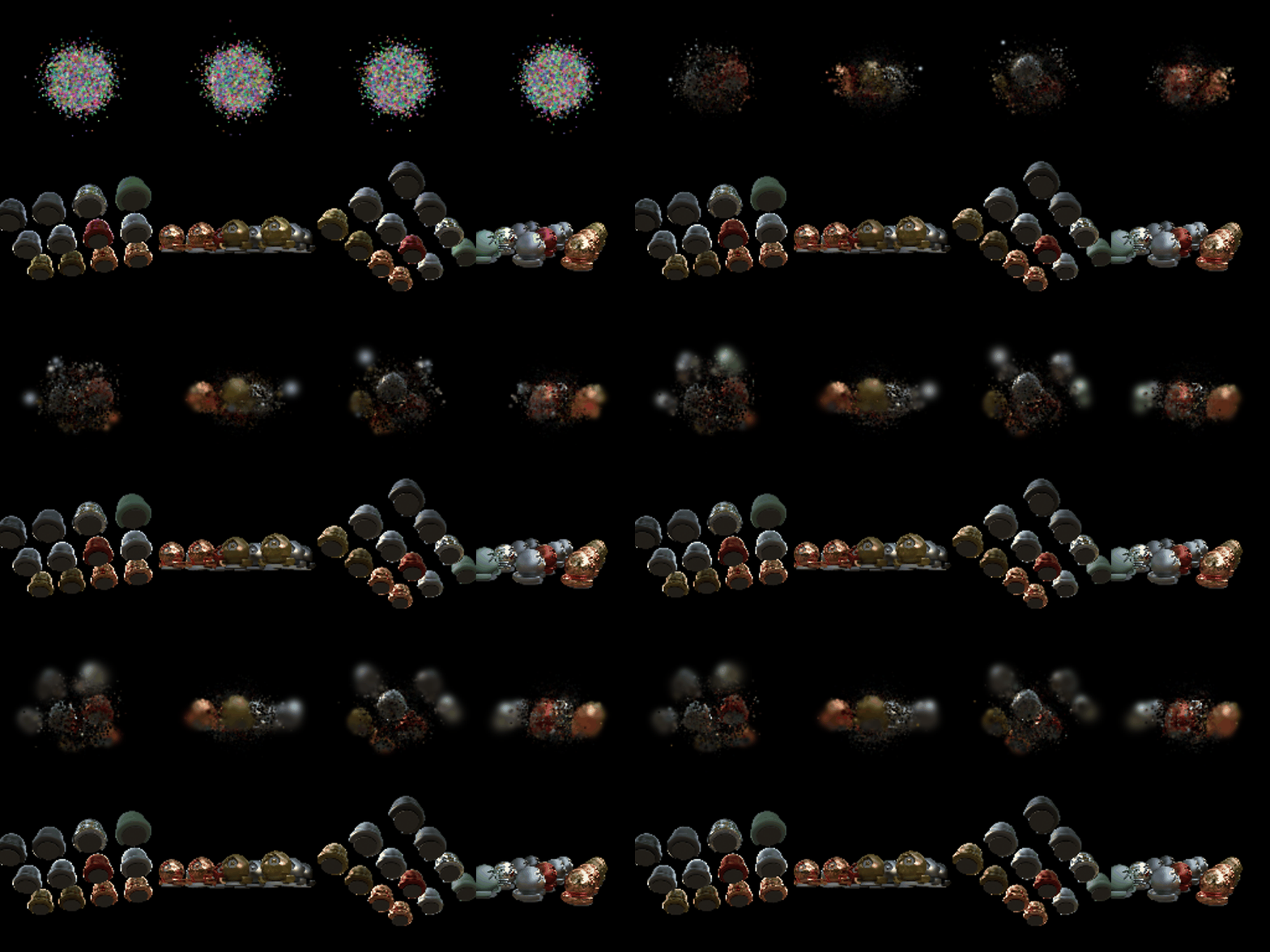
Baseline
Exactly the Q6 setup: isotropic Gaussians, the Q6 learning rates, L1 loss and 1,000
iterations, with init_type="random". The starter draws the means from
N(0, 0.2²I), a small ball at the centre, while the balls of the scene spread over most of
the frame. With a means learning rate of 5e-4, the Gaussians cannot travel that far in 1,000
steps.
Modifications
All changes are behind train_harder_scene.py --improved:
- Spread initialization. The 10,000 random means are redrawn uniformly inside a ball of radius 1.5 that covers the scene, so every ball starts with Gaussians near it instead of having to pull them out of the centre.
- Anisotropic Gaussians. Each Gaussian learns 3 scales and a rotation (quaternion lr 0.001). This lets flat, elongated Gaussians follow the ball surfaces and the ground plane, where isotropic ones need many more.
- L1 + D-SSIM loss, 0.8·L1 + 0.2·(1 − SSIM) as in the 3D Gaussian Splatting paper, with a differentiable SSIM (11×11 Gaussian window). The SSIM term rewards local structure and contrast, which L1 alone treats the same as a flat average.
- Learning rate schedule. Means start at lr 0.002, 4× the Q6 value, so random points can travel to the objects, and decay exponentially to 2e-5 by the end to settle them. Opacities use 0.05; scales and colours keep the Q6 rates.
- Simplified adaptive density control. Every 100 iterations until 70% of training, Gaussians with opacity below 0.005 are removed, and the 5% with the largest average gradient of their mean are cloned, with a random offset of about their own size, up to 30,000. A large mean gradient marks a region that is under-reconstructed. The optimizer is rebuilt after each step because the parameter tensors change. The count grew from 10,000 to 22,137.
- Longer training: 3,000 iterations instead of 1,000. That was about an hour on the 4 GB GPU, since the cost grows with the number of Gaussians.
I changed all of these together and did not run an ablation, so this page does not separate how much each one contributes.