Assignment 1: Rendering Basics with PyTorch3D
1. Practicing with Cameras
1.1 360-degree Renders
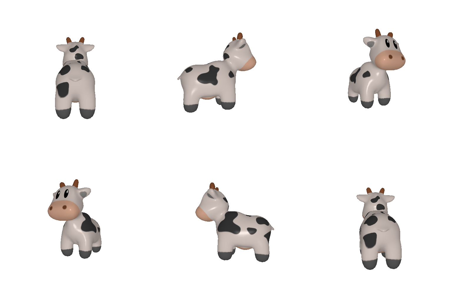
1.2 Re-creating the Dolly Zoom
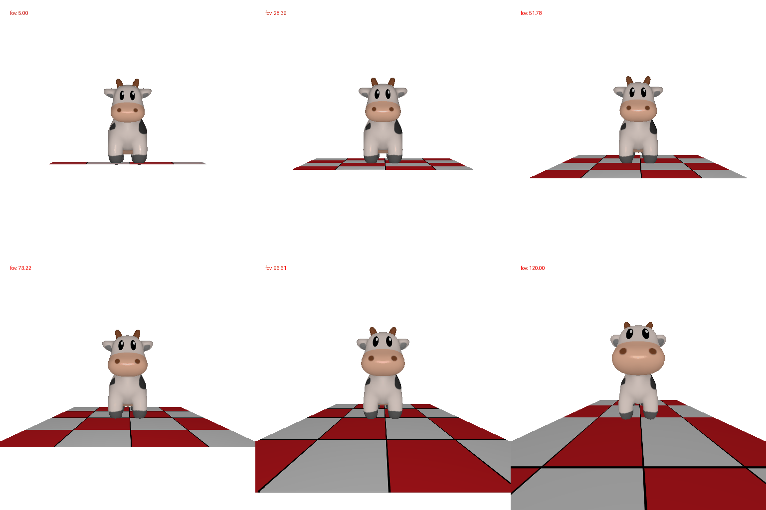
2. Practicing with Meshes
2.1 Constructing a Tetrahedron

The mesh has 4 vertices and 4 triangle faces.
2.2 Constructing a Cube (5 points)
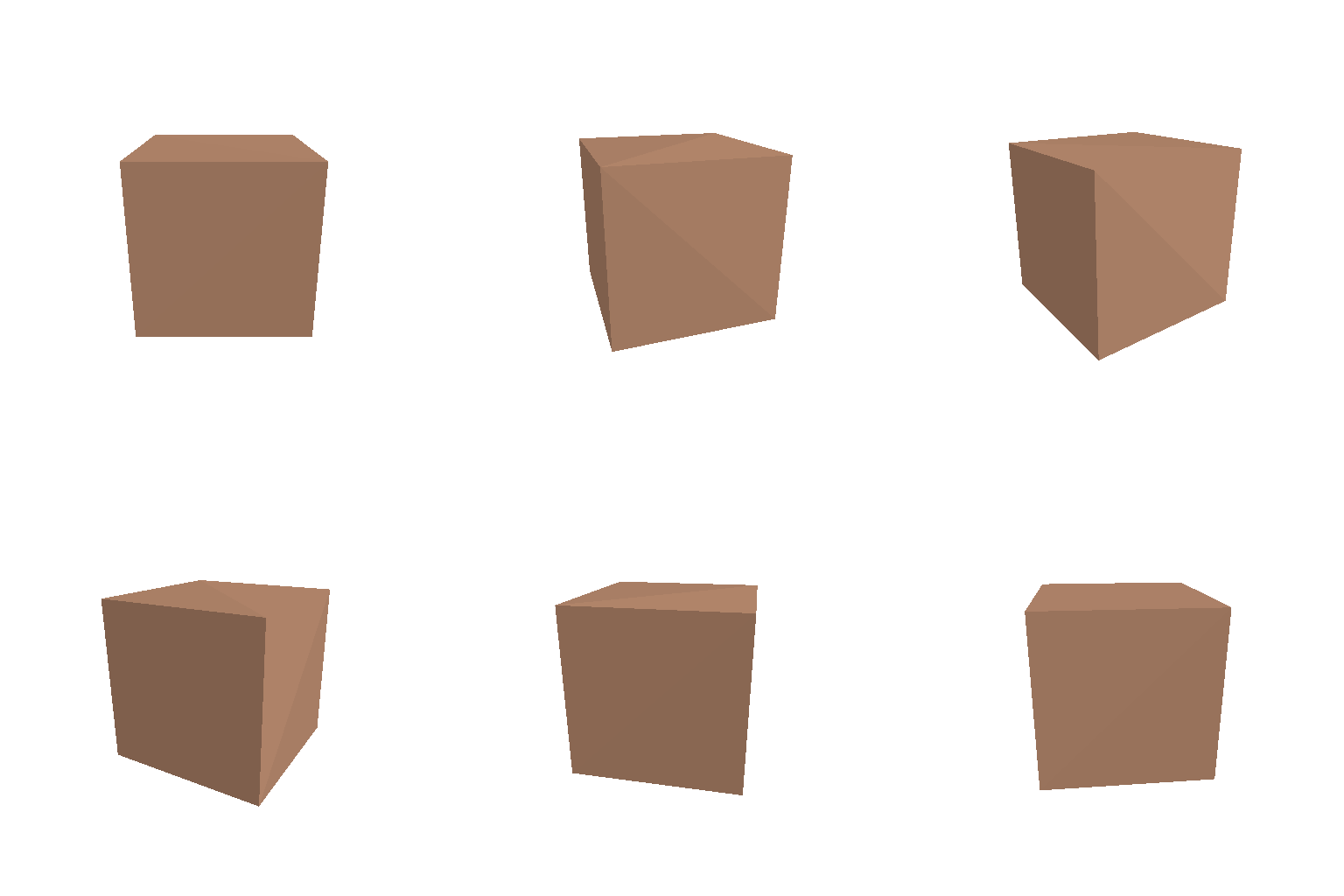
The mesh has 8 vertices and 12 triangle faces.
3. Re-texturing a Mesh

color1 = [0, 0, 1] (blue) on the front, the vertex with the smallest
z, and color2 = [0, 1, 0] (green) on the back, the vertex with the
largest z.
4. Camera Transformations
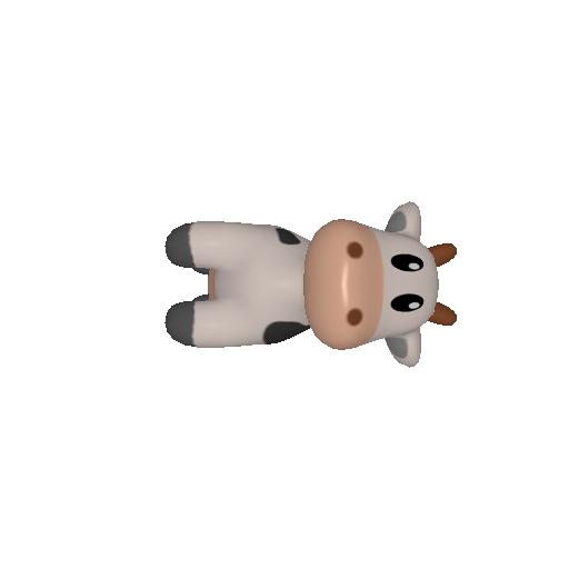
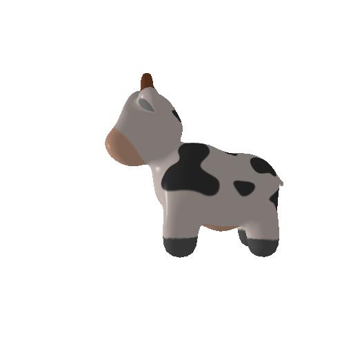
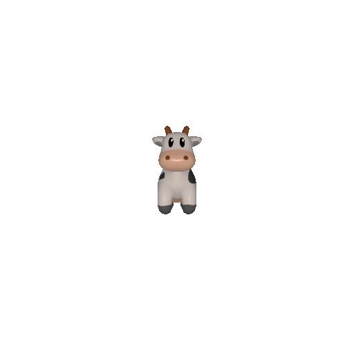
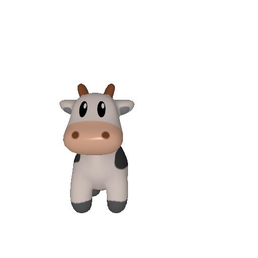
Starting from R_0 = I and T_0 = [0, 0, 3], with
R = R_relative @ R_0 and T = R_relative @ T_0 + T_relative.
R_relative = 90° rotation about z, T_relative = [0, 0, 0].R_relative = 90° rotation about y, T_relative = [-3, 0, 3].R_relative = identity, T_relative = [0, 0, 3].R_relative = identity, T_relative = [0.4, -0.4, 0].
5. Rendering Generic 3D Representations
5.1 Rendering Point Clouds from RGB-D Images
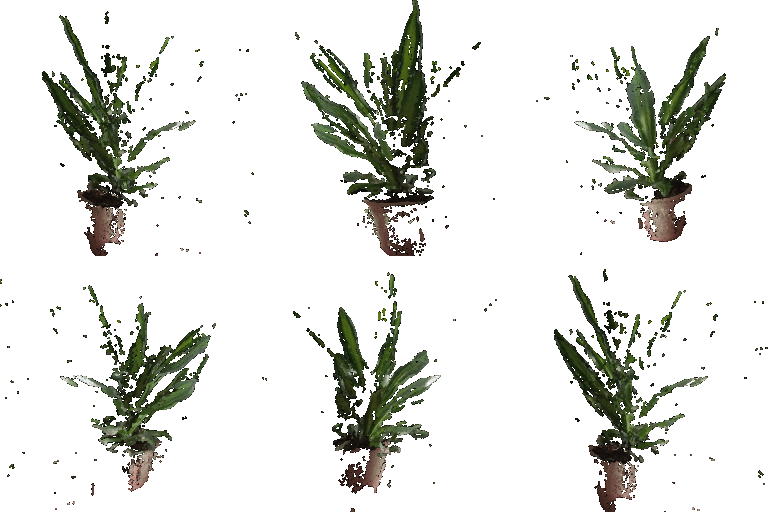
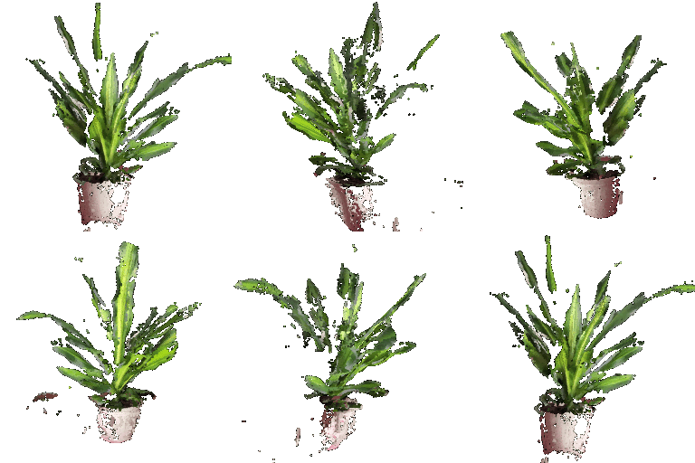
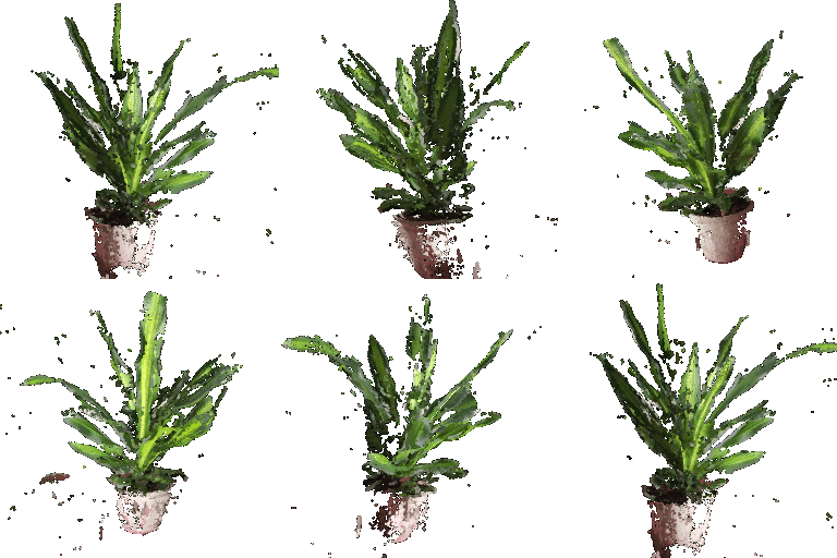
Left to right: the first image, the second image, and the union of the two.
5.2 Parametric Functions
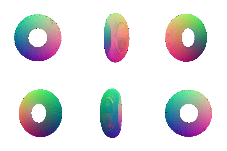
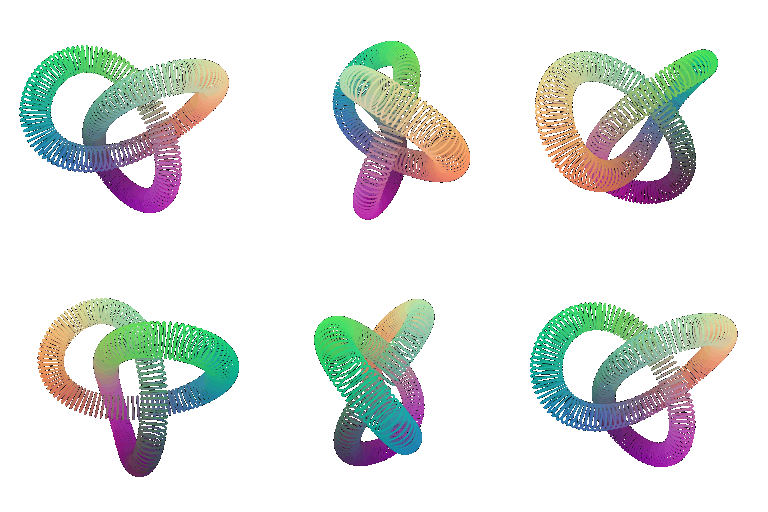
The torus and the trefoil knot
5.3 Implicit Surfaces
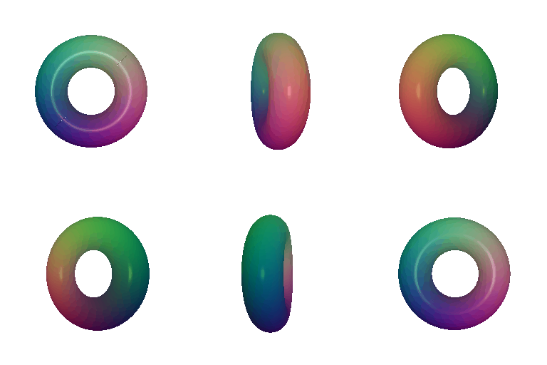
The same torus as a point cloud (5.2, left) and as an implicit surface meshed with
marching cubes (5.3, right).
Mesh vs. point cloud
- Rendering quality. The mesh wins clearly. Because it carries connectivity, it
has surface normals, so it can be shaded and it occludes itself correctly — it reads as a
solid object. The point cloud has no surface between its samples, so its quality depends
entirely on getting the sample count and the splat
radius to match: too small and
the surface is full of pinholes, too large and the silhouette turns into a blobby fringe.
Compare the two gifs above — the mesh has a crisp edge around the hole, the point cloud
does not.
- Rendering speed. Splatting one point is much cheaper than rasterizing and shading
one triangle, but a point cloud needs far more primitives to cover the same surface: the
point cloud above is 40,000 points, the mesh is 36,112 vertices / 72,224 faces yet looks
much denser. The mesh also pays a one-time extraction cost — evaluating the implicit
function on the grid and running marching cubes — before the first frame is drawn.
- Memory. A point cloud stores only positions and colors, with no connectivity
overhead, and scales linearly with however many samples you decide to take. The implicit
route is the expensive one: the voxel grid is O(n³), so 128³ is already ~2M floats
for a surface that only needs ~36K vertices, and doubling the resolution costs 8× the
memory. Once the mesh is extracted, though, it is compact.
- Ease of use. Point clouds are almost free to produce: an RGB-D image unprojects
straight into one (5.1), and any parametric function samples into one (5.2). Meshes need
connectivity, which is exactly what marching cubes is for. Implicit functions are very
pleasant to author and compose — unions, intersections and blends are just min/max on
F — but the topology you get back is limited by the grid: a hole or a tube thinner
than one voxel is simply lost, so the grid resolution silently decides the topology
you end up with. (Neither shape here runs
mcubes.smooth() — both
implicit functions are already continuous fields, and smoothing would only pull the
surface away from the level-set we actually want.)
Goursat's tangle cube
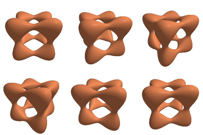
The tangle cube is the zero level-set of
F(x, y, z) = x⁴ − 5x² + y⁴ − 5y² + z⁴ − 5z² + 11.8.
(Extra Credit) 6. Do Something Fun
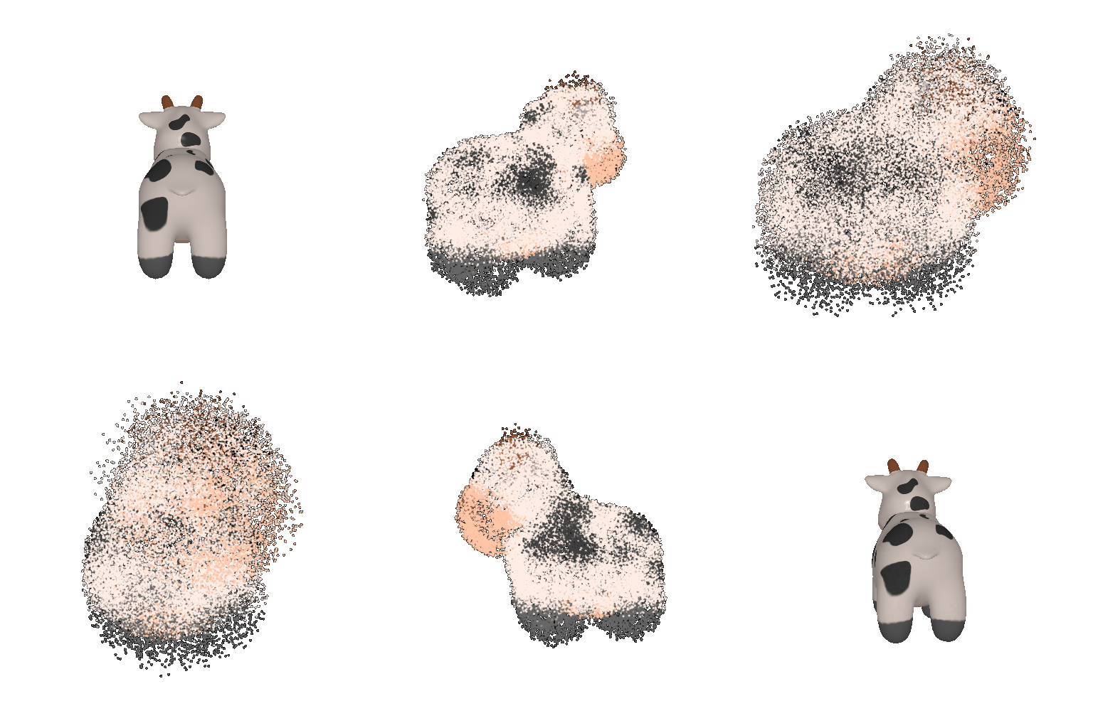
The cow blows apart into a point cloud and puts itself back together
(Extra Credit) 7. Sampling Points on Meshes
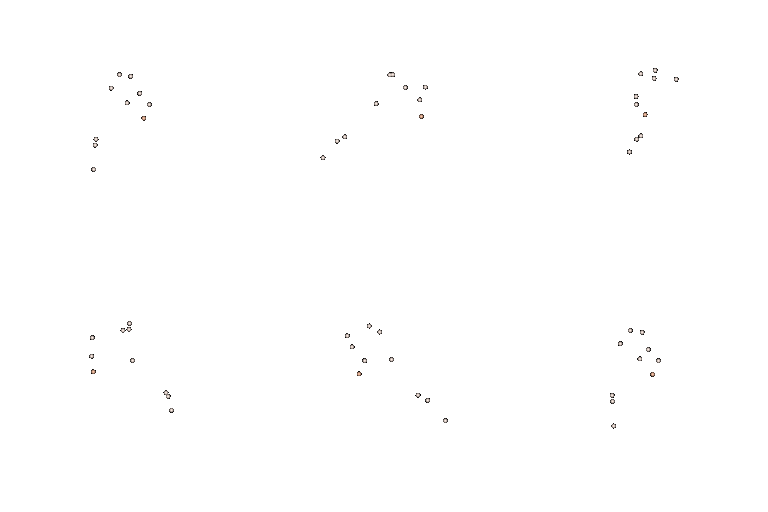
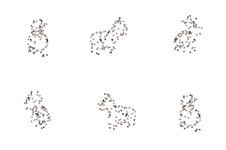
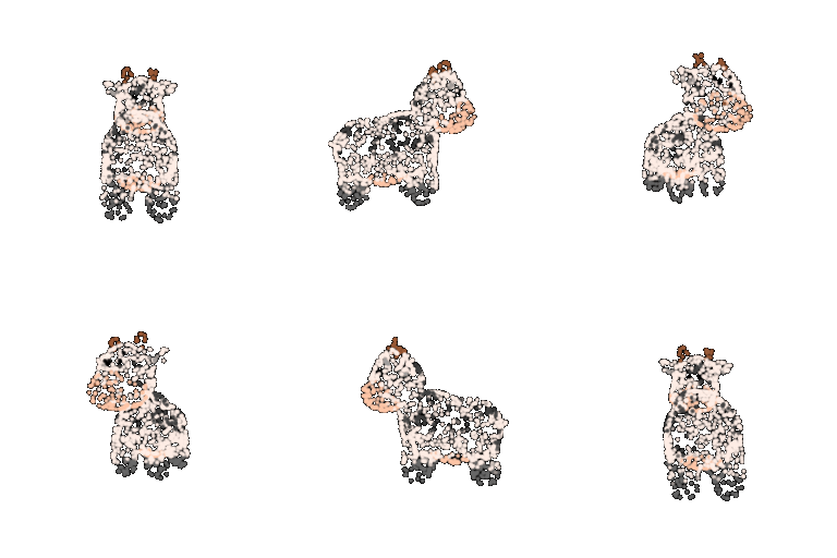
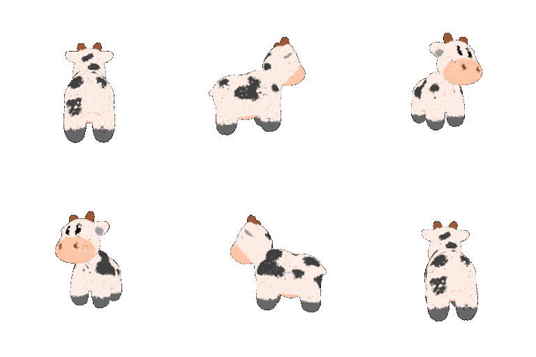
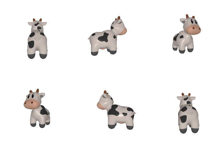
Left to right: 10, 100, 1,000 and 10,000 sampled points, then the original mesh.