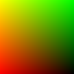
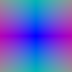
I generated a pixel grid in the range [−1, 1] and used the camera's unprojection function to obtain world-space points. Each ray starts at the camera center and points toward its corresponding image-plane point. I normalized the ray directions to unit length.
| Pixel coordinates | Ray directions |
|---|---|
|
|
I uniformly sampled distances between the near and far bounds. For a ray with origin o and unit direction d, each sample is p(t) = o + t d. The box configuration uses 64 samples per ray over [0, 5]. For the visualization below, I selected every 16th ray to reduce rendering cost.
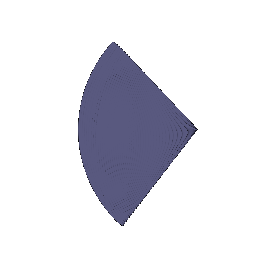
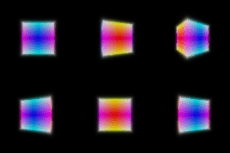
I computed alpha as 1 - exp(-density * delta) and transmittance from the accumulated optical thickness before each sample. The first sample has transmittance 1. Color and depth are weighted sums using the same weights, weight = transmittance * alpha.
| Color rendering | Normalized depth |
|---|---|
 |
 |
The animation contains 20 views at 256 × 256 resolution. I divided the depth image by its maximum value before saving it. The box has a clear outline, with slightly soft edges from the volume representation and finite sampling.
I used torch.randperm to select pixels without replacement within each batch. This allows training on a subset of rays rather than rendering the whole image at every update.
I optimized the box center and side lengths using RGB mean squared error and Adam. Training used 1,000 epochs, 4,096 rays per batch, 64 samples per ray, and learning rate 0.0005.
The learned parameters, rounded to two decimal places, are:
| Parameter | x | y | z |
|---|---|---|---|
| Center | 0.25 | 0.25 | 0.00 |
| Side lengths | 2.01 | 1.50 | 1.50 |

The fitted volume is elongated along one axis and shifted from the origin. The rendered views show a consistent box shape. The last displayed training loss was approximately 0.000001 at epoch 990; this is a batch loss, not a test-set metric.
I used positional encoding with six frequencies and an MLP with six layers, width 128, and an input skip connection at layer index 3. Separate output heads predict density and RGB. ReLU makes density nonnegative, and sigmoid maps RGB to [0, 1]. For this experiment, both outputs depend only on position.
| Setting | Value |
|---|---|
| Dataset | Lego |
| Image resolution | 128 × 128 |
| Training epochs | 250 |
| Rays per batch | 1,024 |
| Samples per ray | 128 |
| Initial learning rate | 0.0005 |
| Final displayed batch MSE | 0.003952 |

The model reconstructs the yellow body, bucket, and tracks from different viewpoints. The geometry and appearance are clearer than in the early training results, although small details remain blurred at this resolution. The reported MSE is from the final training batch, not a held-out evaluation.
This GIF was saved before adding the direction-dependent color branch for Section 4.1.
I kept density dependent only on position. For color, I concatenated the position features with an encoded unit viewing direction. The direction encoding uses two frequencies, and the color branch has a hidden layer of width 64 followed by an RGB output layer and sigmoid.
I trained on the materials dataset for 250 epochs at 128 × 128 resolution, using 1,024 rays per batch, 128 samples per ray, and initial learning rate 0.0001. The final displayed training-batch MSE was 0.005131.
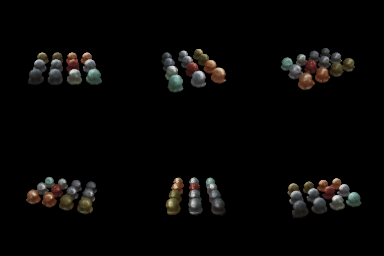
The final rendering separates the objects and their different colors, and shows bright regions on their surfaces. Some surface details remain soft.
View dependence and generalization. A position-only color cannot represent a highlight that changes with viewing direction. Adding direction makes such appearance changes possible, but also gives the network more freedom to fit the training cameras without learning accurate geometry. I limited the direction branch to the color output and used a small direction encoding and hidden layer. These choices restrict its capacity, but do not guarantee better generalization. I did not run a matched position-only materials experiment or a held-out comparison, so the GIF demonstrates the learned result rather than a measured generalization improvement.
I used two networks with independent parameters. The coarse network evaluates 64 uniformly spaced points. I normalize its rendering weights into a probability distribution and sample 64 additional distances using inverse-CDF sampling. The fine network evaluates the sorted union of the original and new points, giving 128 points in total.
Sampling uses detached coarse weights. The training loss is the sum of the coarse and fine RGB MSE losses, so both networks receive supervision. Fine sampling is random during training and deterministic during rendering.
I trained on materials for 250 epochs with the same image resolution, ray batch size, initial learning rate, and view-dependent network design as Section 4.1.
| Single network, uniform sampling | Coarse/fine sampling |
|---|---|
|
 |
Speed and quality. The coarse/fine method uses 64 + 128 = 192 network point evaluations per ray, compared with 128 for the single network. Near the end of training, the single-network logs showed about 39–42 seconds per epoch, while the hierarchical run showed about 71–88 seconds. These were separate runs on the same CPU, not controlled timing benchmarks, and system load may have differed.
The two final animations look similar overall. I did not observe a clear improvement across all views from hierarchical sampling. It allocates more samples to regions with high coarse weights, but requires a second network and additional evaluations. Its benefit also depends on the coarse network locating useful regions. In this experiment, the extra computation did not produce an obvious visual gain. The final hierarchical batch loss was 0.013629, but it sums two MSE terms and cannot be compared directly with the single-network loss. I did not compute held-out NeRF PSNR or MSE.
I computed 3D covariance from scales and quaternion rotations, using a scaled identity matrix for isotropic Gaussians. I then projected the covariance with the supplied projection Jacobian and the camera rotation, and projected the centers into screen coordinates. The 2D Gaussian exponent is computed with a batched quadratic form.
All four provided tests in unit_test_gaussians.py passed.
I transformed Gaussian centers into camera coordinates, removed nonpositive depths, and sorted the remaining Gaussians from near to far. I computed alpha from opacity and the Gaussian exponent, and transmittance with an exclusive cumulative product. Color, depth, and silhouette are accumulated using alpha–transmittance weights. For mini-batches, I passed the transmittance after the last Gaussian to the next batch.
I rendered the pretrained chair using its constant, zero-order color component. Rendering used CPU, a white background, 128 × 128 resolution, and 256 Gaussians per splat. The script enlarges each panel to 256 × 256 for display.

The panels show RGB, depth, and silhouette. The animation contains 32 views. The chair structure and green upholstery are visible, although edges have artifacts and some views crop parts of the chair under the supplied camera path.
I initialized 10,000 isotropic Gaussians from the provided truck point cloud. I optimized their centers, scales, opacities, and colors with Adam. Quaternion rotations stayed fixed because the Gaussians are isotropic.
| Parameter | Learning rate |
|---|---|
| Centers | 0.0001 |
| Pre-activation scales | 0.005 |
| Pre-activation opacities | 0.01 |
| Colors | 0.01 |
The smaller center learning rate limits movement away from the initial point cloud.
I used L1 image loss, a black background, and the original 160 × 90 images. The split contains 197 training views and 5 test views. Rendering uses batches of 128 Gaussians.
I first ran a 100-iteration trial, then trained a fresh model for 1,000 iterations with the same learning rates. The longer run was not resumed from the trial.
| Training iterations | Mean test PSNR (dB) | Mean test SSIM |
|---|---|---|
| 100 | 25.801 | 0.892 |
| 1,000 | 28.863 | 0.933 |
The 1,000-iteration model improves mean PSNR by 3.062 dB and SSIM by 0.041. Its body and wheels are clearer, with fewer colored speckles, although some edges and surface details remain blurred. Since the images contain a large black background, I also inspected foreground quality rather than relying only on the full-image scores.
Training progress. The top row shows predictions and the bottom row shows ground truth. Frames were saved every 50 iterations and at the final iteration.

Final renderings. This animation contains 197 training viewpoints; the quantitative scores above are from the 5 held-out test views.

I loaded the chair's pretrained spherical harmonic coefficients and evaluated the real SH basis through degree 3 using normalized camera-to-Gaussian directions. Each Gaussian has 16 coefficients per color channel, or 48 values in total. I summed the coefficient-weighted basis values, added 0.5, and clamped negative colors to zero. I did not train the SH coefficients.
The SH and constant-color versions use the same 32 camera views, 128 × 128 resolution, and 256 Gaussians per splat. The SH run took 57 minutes 35 seconds on CPU. This is an observed runtime, not evidence that SH itself caused the full rendering cost.
| Zero-order color only (Section 5.5) | Spherical harmonics (Section 7.1) |
|---|---|
|
 |
In the following comparisons, the left image uses only the constant color component and the right image uses SH. Each pair comes from the same frame.
Frame 0. The SH result has a darker green backrest and stronger contrast around the central upholstery pattern. Some areas around the arms are also brighter.

Frame 10. The seat becomes darker and its pattern has stronger contrast. The brightness distribution changes while the overall geometry stays the same.

Frame 28. The underside has a more uniform beige tone, while the surrounding upholstery and frame change in brightness. The differences are more subtle than on the green seat and backrest.

These comparisons show that SH changes appearance with viewing direction. It does not fix the geometric edge artifacts or camera cropping. Without matching ground-truth images for these rendered views, I cannot conclude that every color change is more accurate.