1. Multi-View Data Preprocessing 20 pts
Implement resize_intrinsics, unproject_depth,
canonicalize_cameras, camera_rays and
plucker_coordinates in a4data/geometry.py. Include screenshots of the
data visualizations after unprojection and canonicalization (showing the first camera center
and the valid-point centroid distance), the check_data.py output, and briefly
explain canonicalization, world-space ray directions and the Plücker moment.
Unprojection (original world frame, meters)
Each pixel (u, v) is lifted with X_cam = z · K-1 [u, v, 1]T
(depth is optical-axis z-depth, so no ray normalization), then mapped to the world with the
camera-to-world pose X_world = R X_cam + t. The eight frames of a clip land on one
consistent point cloud.

036bce3393_frame_004470.
076c822ecc_frame_002890.Canonicalization (camera-0 frame, normalized units)
The same scenes after canonicalization. The first camera (red) sits at the origin, about (0, 0, 0), and the valid-point centroid is 1.000 unit away (side panel of each screenshot).

036bce3393_frame_004470: first camera center
(0.0000, 0.0000, 0.0000), scene scale 1.867 m, centroid distance 1.000.
076c822ecc_frame_002890.check_data.py output
python scripts/check_data.py --config configs/scannetpp/iphone/data.json --split train --max-samples 4| Sequence | Views | Res. | Valid depth | Max point reproj. err. (px) | Max ray reproj. err. (px) | Centroid dist. |
|---|---|---|---|---|---|---|
e050c15a8d_frame_007080 | 8 | 224 | 0.978 | 1.07e-4 | 9.31e-5 | 1.0 |
5f99900f09_frame_002820 | 8 | 224 | 0.990 | 1.07e-4 | 9.65e-5 | 1.0 |
47b37eb6f9_frame_002720 | 8 | 224 | 0.961 | 1.10e-4 | 1.08e-4 | 1.0 |
4c5c60fa76_frame_006690 | 8 | 224 | 0.752 | 8.90e-5 | 8.91e-5 | 1.0 |
Batch shapes (batch of 2): rgb, points_world, ray_origins,
ray_directions are (2, 8, 3, 224, 224); depth is
(2, 8, 1, 224, 224); plucker is (2, 8, 6, 224, 224);
original_world_from_reference is (2, 4, 4). All reprojection errors are
about 1e-4 px, far below the 0.01 px threshold.
Explanations
- Canonicalization. Every pose is left-multiplied by the inverse of camera 0's
pose,
T'i = T0-1 Ti, so camera 0 becomes the identity and the scene is expressed in its frame. Translations, depths and points are then divided by the scene scale (the distance from camera 0 to the valid-point centroid), so the centroid ends up exactly 1 unit away. This removes the arbitrary world origin, orientation and metric scale that a model cannot infer from images alone; rotations are unchanged by the scaling. - World-space ray directions. A pixel's camera-space direction is
K-1 [u, v, 1]T. Only the rotation applies to directions:d = normalize(R K-1 [u, v, 1]T); the translationtis the ray origin (the camera center), shared by all pixels of a view. - Plücker moment.
m = o × dis perpendicular to the plane through the world origin and the ray, and its magnitude is the ray's distance from the origin. Unlike the origino, it is the same for every point on the ray ((o + s d) × d = o × d), so[d, m]describes the ray itself uniquely, independent of where along it the origin is chosen.
2.1 Mini-LVSM Overfitting 10 pts
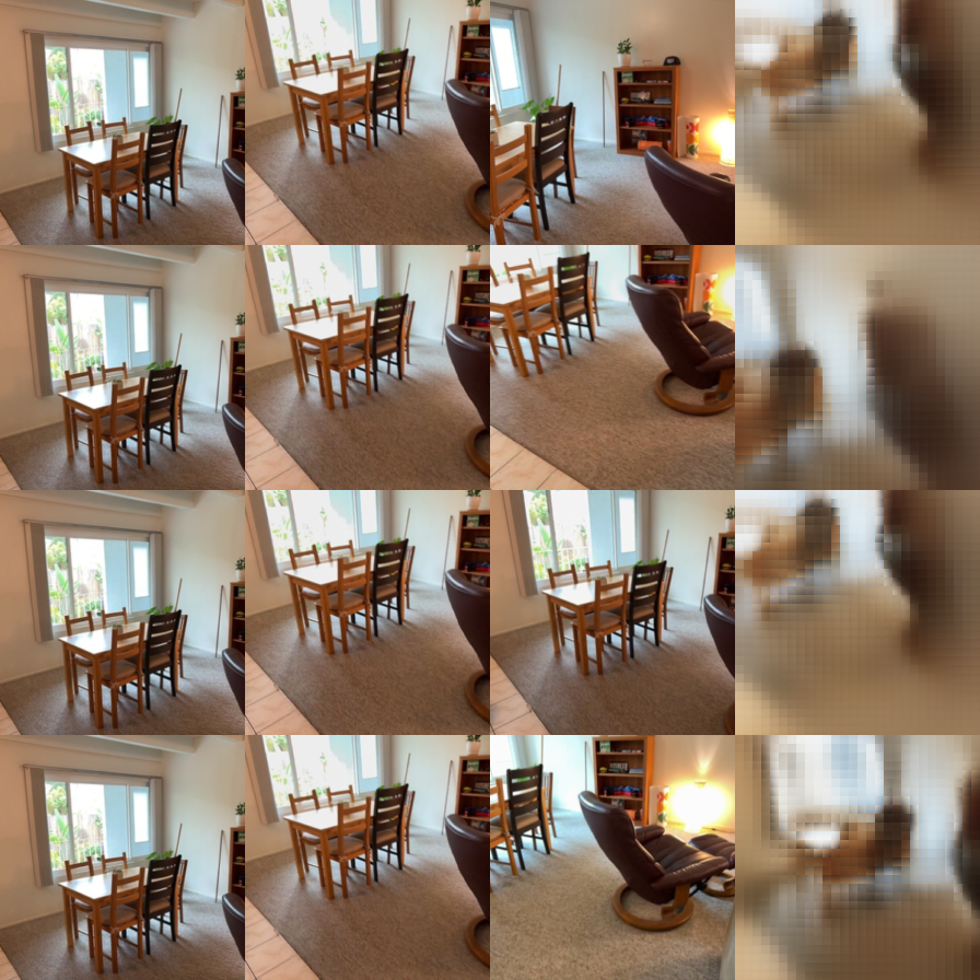
Overfit one fixed batch (--overfit 2000). Include the final overfit PSNR and the
val_epoch000.png visualization.
After 2000 steps on one batch, the final overfit PSNR is 30.96 dB (SSIM 0.871, MSE 8.6e-4), above the ~30 dB target.

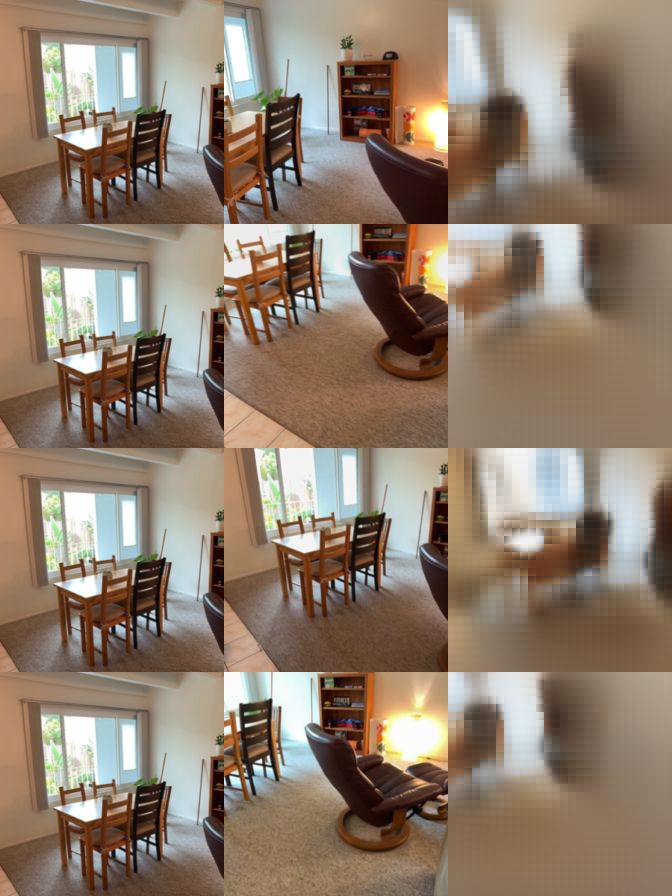
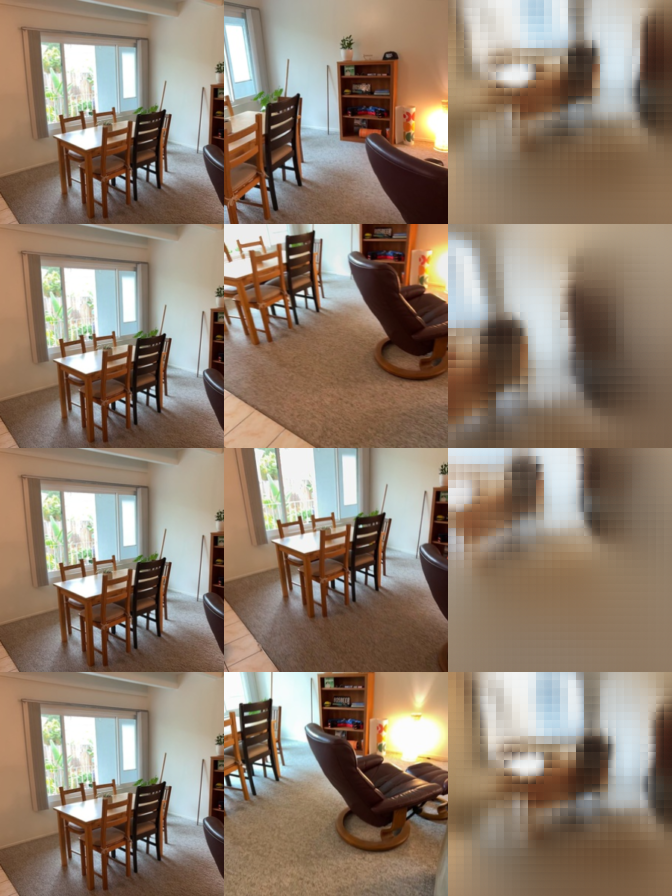
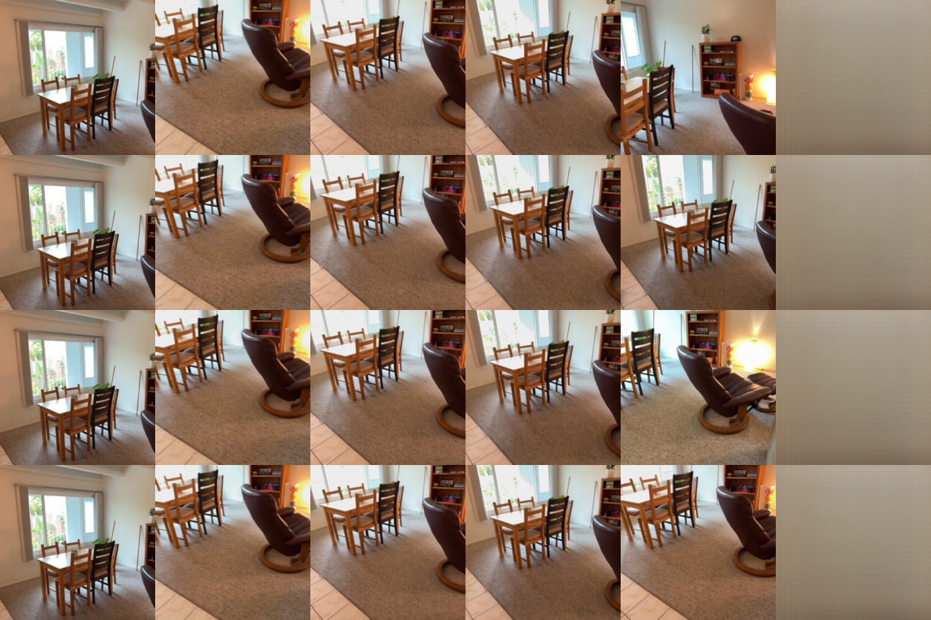
val_epoch000.png after overfitting. Columns: source views, ground truth, prediction.2.2 Mini-LVSM Training and Evaluation 30 pts
Train on the full training split and evaluate best.pt with 1, 2 and 4 source views
and correct / shuffled / no target-ray conditioning. Include training curves, PSNR/SSIM for each
setting, training and evaluation visualizations, the training settings, and discuss the effect
of the number of source views and of the ray conditioning.
Training settings
Mini-LVSM (14.6M parameters): patch size 8, width 384, 8 transformer blocks, head dimension 64, MLP ratio 4, QK-norm. AdamW (lr 2e-4, weight decay 0.05, betas 0.9/0.95), 200 warmup steps then cosine decay to 10%, gradient clipping 1.0, bf16 autocast. Batch size 4, 8 views per clip at 224×224 (2 source + 6 target views), sampling range 32. I trained the default 100 epochs first (53 min), and since validation PSNR was still rising, a second run for 300 epochs (56 steps/epoch, 2.6 h on a 16 GB laptop GPU). Results below use the 300-epoch run (best validation PSNR at epoch 297).


Ablations (validation, 300-epoch best.pt)
python -m models.lvsm.eval --checkpoint outputs/lvsm_long/best.pt --num-source-views 1 2 4 --conditioning correct shuffled none| Source views | Correct rays PSNR / SSIM | Shuffled rays PSNR / SSIM | No rays PSNR / SSIM |
|---|---|---|---|
| 1 | 15.77 / 0.582 | 11.66 / 0.483 | 12.48 / 0.534 |
| 2 | 16.94 / 0.591 | 11.26 / 0.464 | 12.42 / 0.530 |
| 4 | 18.07 / 0.610 | 11.36 / 0.463 | 12.43 / 0.540 |
For comparison, the 100-epoch model with correct rays scores 15.20 / 16.14 / 16.88 dB for 1 / 2 / 4 source views.
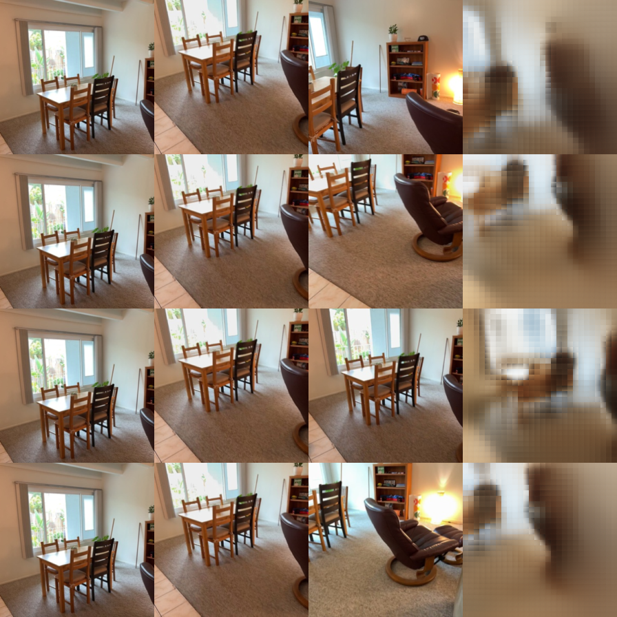
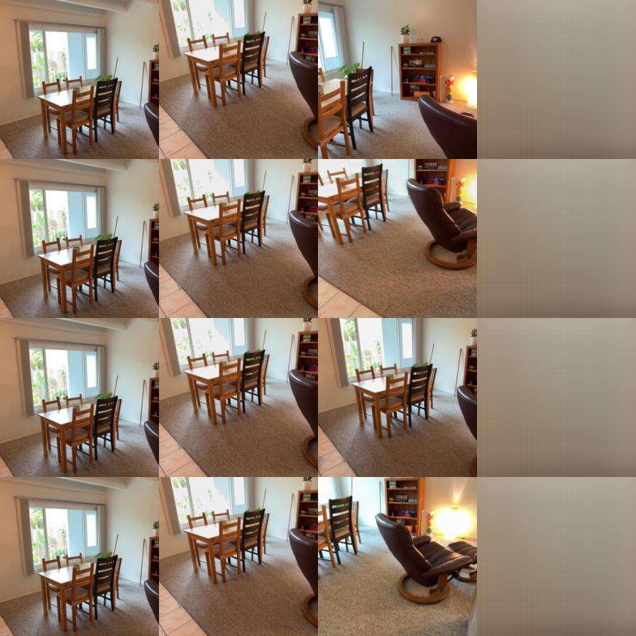
Training visualizations


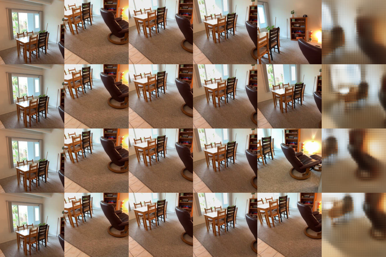
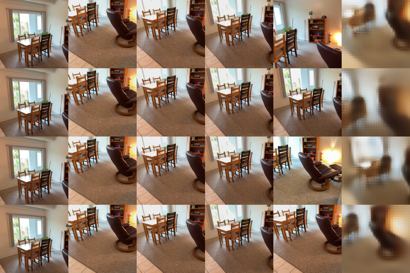
Evaluation visualizations
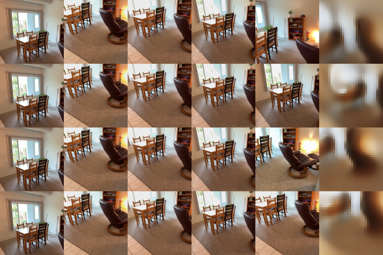
Columns: source views, ground truth, prediction.
Discussion
- Number of source views. With correct rays, PSNR rises steadily with more sources: 15.8 → 16.9 → 18.1 dB for 1 → 2 → 4 views, even though the model was trained only with 2. More sources cover more of the scene, so less of the target has to be guessed, and attention generalizes to longer token sequences without retraining.
- Ray conditioning. Shuffled rays drop PSNR by 4–7 dB, to about 11.3–11.7 dB, below even the no-ray setting (about 12.4 dB). With zero rays the model has no viewpoint and falls back to a blurry "average" view near the sources, which is safe under MSE. With shuffled rays it confidently renders another target's viewpoint, so the content is misaligned and is penalized more. The no-ray result is also flat across S, since without a query pose extra sources do not help. This shows that the model really uses the Plücker target rays.
- Limitations. Predictions are blurry and show patch-grid artifacts: the model is small, trained briefly, and the MSE loss favors averaging over uncertain detail.
2.3 Bonus: Mini-LVSM Exploration 10 pts
Describe your question, experimental settings, results and conclusions, with plots or screenshots, possible explanations and limitations.
Question: does training with a random number of source views help?
The Q2.2 model is always trained with S = 2 sources, yet it is evaluated with 1, 2 and 4. I tested whether exposing the model to every evaluation setting during training, by drawing S uniformly from {1, 2, 3, 4} at each step (the remaining 8 − S views are targets), improves the 1- and 4-view results without hurting 2 views.
Setup
A controlled comparison against the default 100-epoch S = 2 run: identical model, optimizer,
schedule, data, seed and epoch count (100 epochs, 56 steps/epoch); only the per-step S differs.
Validation during training still uses S = 2, and both best.pt checkpoints are evaluated
with the same Q2.2 command. Change: about five lines in train_one_epoch, enabled by
"random_source_views": [1, 4] in configs/lvsm_randS.json. Cost: 33 s/epoch
vs 32 s/epoch.
python -m models.lvsm.train --config configs/lvsm_randS.json
python -m models.lvsm.eval --checkpoint outputs/lvsm_randS/best.pt --num-source-views 1 2 4 --conditioning correct shuffled none
Results (validation, correct rays)
| Source views at eval | Fixed S = 2 PSNR / SSIM | Random S ∈ {1..4} PSNR / SSIM | Δ PSNR |
|---|---|---|---|
| 1 | 15.20 / 0.558 | 15.28 / 0.560 | +0.08 |
| 2 | 16.14 / 0.560 | 16.24 / 0.560 | +0.10 |
| 4 | 16.88 / 0.575 | 17.08 / 0.575 | +0.20 |
The ray ablations behave as before for the random-S model: shuffled rays give 11.4–11.8 dB and no rays about 12.5 dB at every S.

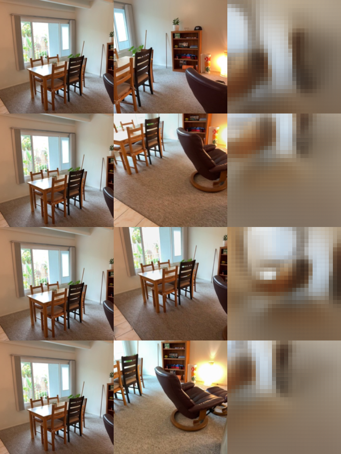
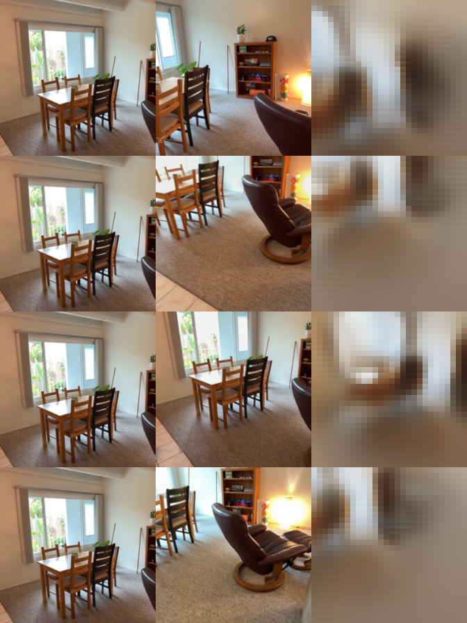

Conclusions and limitations
- Random-S training is slightly better at every evaluation setting, and the gain is largest where the train/test mismatch is largest, at 4 views (+0.20 dB). It costs nothing at S = 2, even though the model now spends only a quarter of its steps on S = 2.
- The effect is small. The fixed-S model already generalizes well to other S, because the transformer treats sources as an unordered set of tokens with no view-index embedding, so attention extends naturally to more or fewer source tokens. Changing S mainly changes how many tokens there are, not what they mean.
- Visually the two models are nearly indistinguishable; both remain blurry, which is limited by model size and training length rather than by the source-view schedule.
- Limitations: a single seed per setting, so differences of ~0.1 dB are within run-to-run noise; and only 100 epochs. Steps with S = 4 also supervise only 4 targets instead of 6, so the random-S model sees slightly fewer target images in total; a longer run may show a larger benefit.
3.1 Mini-VGGT Overfitting 10 pts
Overfit one fixed training clip. Include the overfit loss curve (total, camera and depth loss) and screenshots comparing GT and predicted geometry.
After 40 epochs × 25 steps on one clip, the camera loss falls to 0.0025 and the depth loss
goes negative (the confidence term −0.2 log c lets it drop below zero). On the fitted clip:
rotation error 0.22°, translation error 0.42°, pose AUC@30 0.995, depth AbsRel 0.036,
δ1 0.957. The predicted geometry closely matches GT.


3.2 Mini-VGGT Training and Evaluation 30 pts
Train on the full training split and evaluate best.pt on validation and test.
Include the loss curve, validation/test metrics, GT/prediction screenshots for four different
scenes, the training settings, and discuss errors on held-out scenes.
Training settings
Default configs/vggt.json: frozen DINOv2 ViT-B/14 encoder, 8 frame/global attention
pairs (width 384, 6 heads), camera head with 4 cross-view blocks, depth head with RGB refinement.
Loss weights camera 5.0, depth 1.0. AdamW, lr 6e-4, weight decay 0.01, 10 warmup epochs then
cosine decay to 5%, bf16. Batch size 16, 8 views, sampling range 32, 224×224, seed 825,
1000 epochs (14 steps/epoch). Training took 6.5 h on a single 16 GB laptop GPU.
best.pt (lowest validation loss) is from epoch 929.

Metrics
python -m models.vggt.eval --checkpoint outputs/vggt_train/best.pt --split {val,test} --eval-root data/scannetpp/prepared_eval \
--num-views 8 --eval-num-frames 32 --image-size 224 --seed 825| Metric | Validation (28 scenes) | Test (28 scenes) |
|---|---|---|
| Total / camera / depth loss | 0.789 / 0.112 / 0.231 | 0.759 / 0.100 / 0.260 |
| Depth AbsRel ↓ | 0.127 | 0.151 |
| Depth RMSE (normalized) ↓ | 0.176 | 0.193 |
| Depth δ1 ↑ | 0.861 | 0.821 |
| Mean rotation error ↓ | 12.24° | 10.92° |
| Mean translation-direction error ↓ | 42.43° | 42.02° |
| Rotation AUC @5 / 15 / 30 ↑ | 0.187 / 0.505 / 0.696 | 0.180 / 0.473 / 0.674 |
| Translation AUC @5 / 15 / 30 ↑ | 0.015 / 0.082 / 0.192 | 0.012 / 0.063 / 0.171 |
| Joint pose AUC @5 / 15 / 30 ↑ | 0.003 / 0.057 / 0.166 | 0.002 / 0.045 / 0.153 |
GT vs prediction, four validation scenes

09c1414f1b, GT.
09c1414f1b, prediction.
21d970d8de, GT.
21d970d8de, prediction.
280b83fcf3, GT.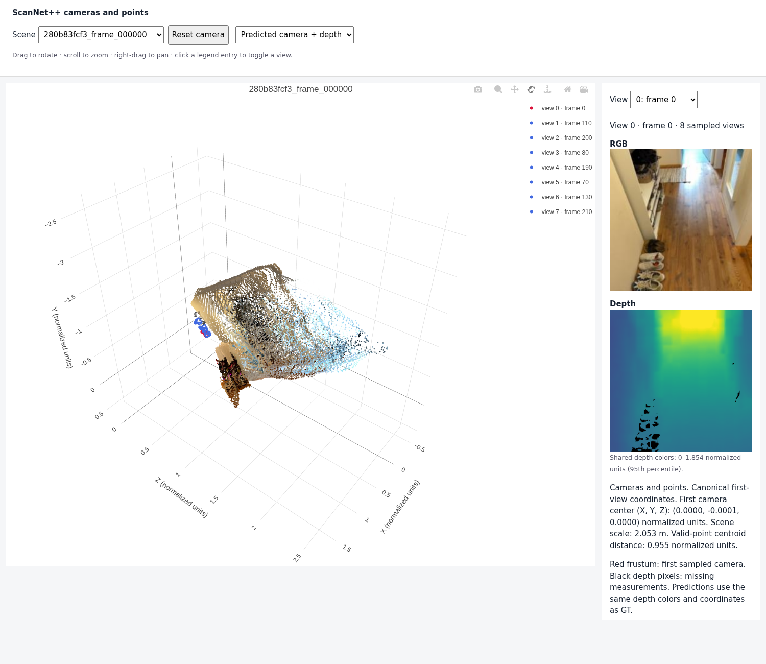
280b83fcf3, prediction.
2b1dc6d6a5, GT.
2b1dc6d6a5, prediction.Discussion of held-out errors
- Depth is the strongest output. 82–86% of valid pixels are within 25% of the
true depth, and the predicted point clouds recover the overall room layout (walls, floor,
furniture). The predictions are much smoother than GT: flat walls become rounded blobs and
sharp corners are lost (e.g. the hallway in
280b83fcf3, Figures 19–20, where the far end of the corridor is also pulled closer and scattered). - Rotation is reasonable, translation is the weak point. Mean rotation error is about 11–12° with rotation AUC@30 near 0.68, but the translation-direction error is about 42° and its AUC@30 is under 0.2, which also caps the joint pose AUC. Frames come from a 32-frame window of a handheld video, so baselines are short; for small baselines the translation direction is poorly constrained by appearance, and small errors in camera positions near each other become large angular errors.
- Generalization. Validation and test numbers are close (test is slightly worse on depth, slightly better on rotation), so the model is not overfit to the validation scenes. The train loss stays above the validation loss, likely because training clips are sampled with random view orders from anywhere in each sequence, while validation uses fixed views from the first 32 frames.
- Room for improvement. Validation loss was still slowly improving at the end, so longer training, a larger model, or fine-tuning DINO would likely help, particularly for camera translation.
3.3 Bonus: Mini-VGGT Exploration 10 pts
Describe your question, experimental settings, results and conclusions, with plots or screenshots, possible explanations and limitations.
Question: direct point-map prediction vs camera + depth
The baseline reconstructs 3D points by unprojecting predicted depth with predicted cameras. I added a head that predicts canonical world-space points directly, trained it jointly with the camera and depth heads, and asked two things: (1) which point map is more accurate, and (2) does the extra point supervision change camera and depth quality (multi-task effect)?
Implementation
PointHeadmirrorsDepthHeadwith three output channels: a per-patch linear decoder to 14×14×3 values, then a two-layer 3×3 conv residual conditioned on RGB. No output activation, since canonical coordinates can be negative.point_loss: trimmed mean (98%) of the per-pixel L2 point error over GT-valid pixels, plus the multi-scale gradient loss applied to each coordinate channel. Added to the total with weight 1.0 (camera 5.0, depth 1.0 unchanged).- Everything else matches Q3.2: same data, seed, batch size 16, 1000 epochs, optimizer and
schedule. To fit the extra head in 16 GB, the first 4 of the 16 aggregator blocks use gradient
checkpointing; this only trades compute for memory and does not change the computation.
Training took 7.5 h.
best.ptis from epoch 985. scripts/compare_points.pymeasures, over all GT-valid pixels, the mean L2 error of each point map against GT points. It also unprojects predicted depth with the GT cameras, which separates depth error from camera error.
python -m models.vggt.train --config configs/vggt_points.json --output outputs/vggt_points
python scripts/compare_points.py --checkpoint outputs/vggt_points/best.pt --split {val,test} --eval-root data/scannetpp/prepared_eval \
    --num-views 8 --eval-num-frames 32 --image-size 224 --seed 825
Results: point-map accuracy
Mean L2 point error, normalized units (meters in parentheses). Lower is better.
| Points from | Baseline (Q3.2), val | + point head, val | Baseline (Q3.2), test | + point head, test |
|---|---|---|---|---|
| Point head (direct) | — | 0.265 (0.549 m) | — | 0.242 (0.470 m) |
| Predicted cameras + predicted depth | 0.248 (0.501 m) | 0.260 (0.533 m) | 0.251 (0.491 m) | 0.231 (0.444 m) |
| GT cameras + predicted depth | 0.128 (0.281 m) | 0.136 (0.301 m) | 0.142 (0.287 m) | 0.146 (0.288 m) |
Results: effect on camera and depth
| Metric | Baseline, val | + points, val | Baseline, test | + points, test |
|---|---|---|---|---|
| Depth AbsRel ↓ | 0.127 | 0.139 | 0.151 | 0.151 |
| Depth δ1 ↑ | 0.861 | 0.844 | 0.821 | 0.808 |
| Rotation error ↓ | 12.24° | 12.19° | 10.92° | 10.30° |
| Translation error ↓ | 42.43° | 42.51° | 42.02° | 38.45° |
| Rotation AUC@30 ↑ | 0.696 | 0.702 | 0.674 | 0.705 |
| Translation AUC@30 ↑ | 0.192 | 0.184 | 0.171 | 0.194 |
| Pose AUC@5 / 15 / 30 ↑ | 0.003 / 0.057 / 0.166 | 0.007 / 0.061 / 0.167 | 0.002 / 0.045 / 0.153 | 0.004 / 0.059 / 0.179 |


280b83fcf3, predicted cameras + depth.
280b83fcf3, point head.
09c1414f1b, predicted cameras + depth.
09c1414f1b, point head.GT for these scenes is in Figures 15 and 19.
Conclusions
- Camera + depth beats direct points, slightly. Within the same model, unprojecting predicted depth with predicted cameras is 2–5% more accurate than the point head (0.260 vs 0.265 val, 0.231 vs 0.242 test). The factored form builds in the projective structure: depth is a per-pixel scalar along a known ray, so the network only has to learn one number per pixel plus a few camera parameters shared by all pixels. The point head has to output all three coordinates and learn the ray geometry implicitly. Visually its clouds are rounder and blurrier, for example the hallway walls in Figure 30.
- Camera error dominates the point error either way. With GT cameras the error roughly halves (about 0.13–0.15), so better poses, especially translation, matter more than better depth or a different point representation.
- Multi-task effect: mixed, slightly helps cameras, slightly hurts depth. On test the joint model has clearly better poses (translation error 42.0° → 38.4°, pose AUC@30 0.153 → 0.179), and its validation camera loss drops faster early in training. Point maps live in the shared camera-0 frame, so supervising them gives the shared features a direct cross-view geometric signal. On validation the camera metrics are essentially unchanged, and depth is slightly worse on both splits (δ1 −0.013 to −0.017), which is consistent with the heads competing for the same feature capacity.
- Limitations. One seed per model and 28 scenes per split, so val/test differences of this size (e.g. the test-only pose gain) may partly be noise. I did not tune the point-loss weight or add a confidence output to the point head as full VGGT does, either of which could change the balance between tasks.