1.3 Ray Sampling 5 pts
Implement get_pixels_from_image and get_rays_from_pixels in
ray_utils.py, and visualize xy_grid and the rays with
vis_grid / vis_rays.
Pixel coordinates are mapped to NDC in [-1, 1] on both axes. Each NDC point is
placed on the image plane at depth 1, unprojected to world space, and the ray direction is
the normalized vector from the camera center to that point:
x, y = torch.arange(W), torch.arange(H)
x, y = x / (W - 1) * 2 - 1, y / (H - 1) * 2 - 1

ndc_points   = cat([xy_grid, ones], -1)        # z = 1
world_points = camera.unproject_points(ndc_points, world_coordinates=True, from_ndc=True)
rays_o = camera.get_camera_center().expand(N, -1)
rays_d = F.normalize(world_points - rays_o, dim=-1)
xy_grid visualization.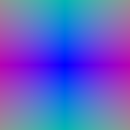
|d| as RGB).1.4 Point Sampling 5 pts
Implement StratifiedRaysampler in sampler.py and visualize the
sample points from the first camera with render_points.
Depths are spaced uniformly between min_depth and max_depth and
broadcast against every ray to get an (N, P, 3) tensor of sample points:
z_vals = torch.linspace(min_depth, max_depth, n_pts_per_ray).view(1, -1, 1) # (1, P, 1)
sample_points = origins[:, None, :] + directions[:, None, :] * z_vals       # (N, P, 3)
sample_lengths = z_vals * ones_like(sample_points[..., :1])                 # (N, P, 1)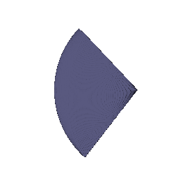
1.5 Volume Rendering 20 pts
Implement VolumeRenderer._compute_weights and _aggregate, and
render a depth map in addition to color. Visualize the spiral rendering and the depth
(normalized by its maximum).
Transmittance at sample i is an exclusive running product, which I compute in parallel as a cumulative sum in log space instead of looping over samples:
sd = density * deltas                                      # (N, P, 1)
sd_excl = cat([zeros_like(sd[:, :1]), sd[:, :-1]], dim=1)  # shift right: T_0 = 1
T = exp(-cumsum(sd_excl, dim=1))
weights = T * (1 - exp(-density * deltas))

feature = sum(weights * rays_feature, dim=1)               # (N, P, C) -> (N, C)
depth   = sum(weights * depth_values, dim=1)               # expected depth
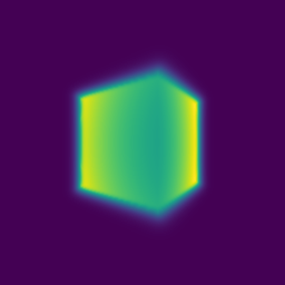
2. Optimizing a Basic Implicit Volume 10 pts
(2.1) Implement random ray subsampling in get_random_pixels_from_image.
(2.2) Use an MSE loss to optimize the box's center and side lengths, and report them
rounded to two decimals. (2.3) Attach the spiral rendering of the optimized volume.
# 2.1: random subset of pixels per iteration
idx = torch.randperm(xy_grid.shape[0])
xy_grid_sub = xy_grid[idx][:n_pixels]

# 2.2: MSE between rendered and ground-truth colors
loss = criterion(rgb_gt, out['feature'])| x | y | z | |
|---|---|---|---|
| Box center | 0.25 | 0.25 | 0.00 |
| Box side lengths | 2.01 | 1.50 | 1.50 |
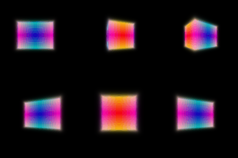
3. Optimizing a Neural Radiance Field 20 pts
Implement the NeRF MLP in NeuralRadianceField (density via ReLU, color via
Sigmoid, optional positional encoding), fill in the loss in train_nerf, and
train on the lego bulldozer (--config-name=nerf_lego).
Sample points are positionally encoded (6 frequencies, 39 dimensions) and passed through
the provided MLPWithInputSkips trunk: 6 layers, 128 hidden units, with the
encoding concatenated back in before layer 3 as in the NeRF paper. Two small heads read the
trunk features:
h = MLPWithInputSkips(n_layers=6, input_dim=39,
                      hidden_dim=128, input_skips=[3])(emb, emb)
density = ReLU(Linear(128, 1)(ReLU(h)))                               # density >= 0
color   = Sigmoid(Linear(64, 3)(ReLU(Linear(128, 64)(ReLU(h)))))      # color in [0, 1]

loss = mse_loss(out['feature'], rgb_gt)
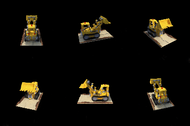
Trained for 250 epochs on 128×128 images, 128 samples per ray. Test-set PSNR: 24.51 dB.
4.1 View Dependence 10 bonus
Make emission depend on viewing direction, show results on the materials scene, and discuss the trade-off between view dependence and generalization.
The ray direction is encoded (2 frequencies) and concatenated with the trunk features only at the input of the color head; density still depends on position alone. Letting density see the direction would let the network explain each training view with different geometry.
dir_emb = harmonic_embedding_dir(normalize(rays_d))          # (N, D)
dir_emb = dir_emb[:, None].expand(N, P, -1).reshape(N * P, -1)
density = density_head(h)                                    # position only
color   = color_head(cat([ReLU(h), dir_emb], -1))            # position + direction
Training stabilizer. On the materials scene, my first view-dependent
runs collapsed. Every density pre-activation went negative (max −0.02), so the ReLU
gave zero density and zero gradient everywhere, and the model rendered all black (test
PSNR 14.3 dB). The scene is mostly black background, so "no density anywhere" is an easy
early local minimum. I kept the required ReLU and added NeRF-style Gaussian noise to the raw
density during training only (density_noise_std = 1.0, the config field that
already existed), and used the same setting for every row below so they are comparable.
| Model (materials, 250 epochs) | Train PSNR | Test PSNR | (Train - Test) gap |
|---|---|---|---|
| View-independent (Q3 model) | 23.43 | 23.16 | 0.27 |
| View-dependent, 2 direction frequencies | 24.25 | 23.57 | 0.68 |
| View-dependent, 6 direction frequencies | 24.31 | 23.53 | 0.78 |
| View-dependent, 2 frequencies, 400×400 | 24.51 | 23.71 | 0.80 |

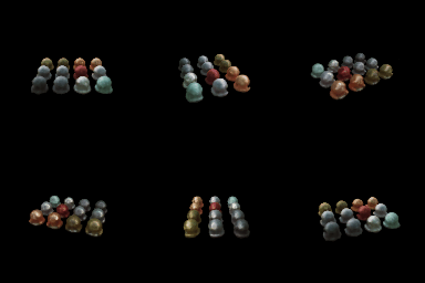
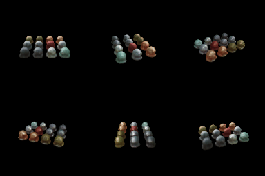
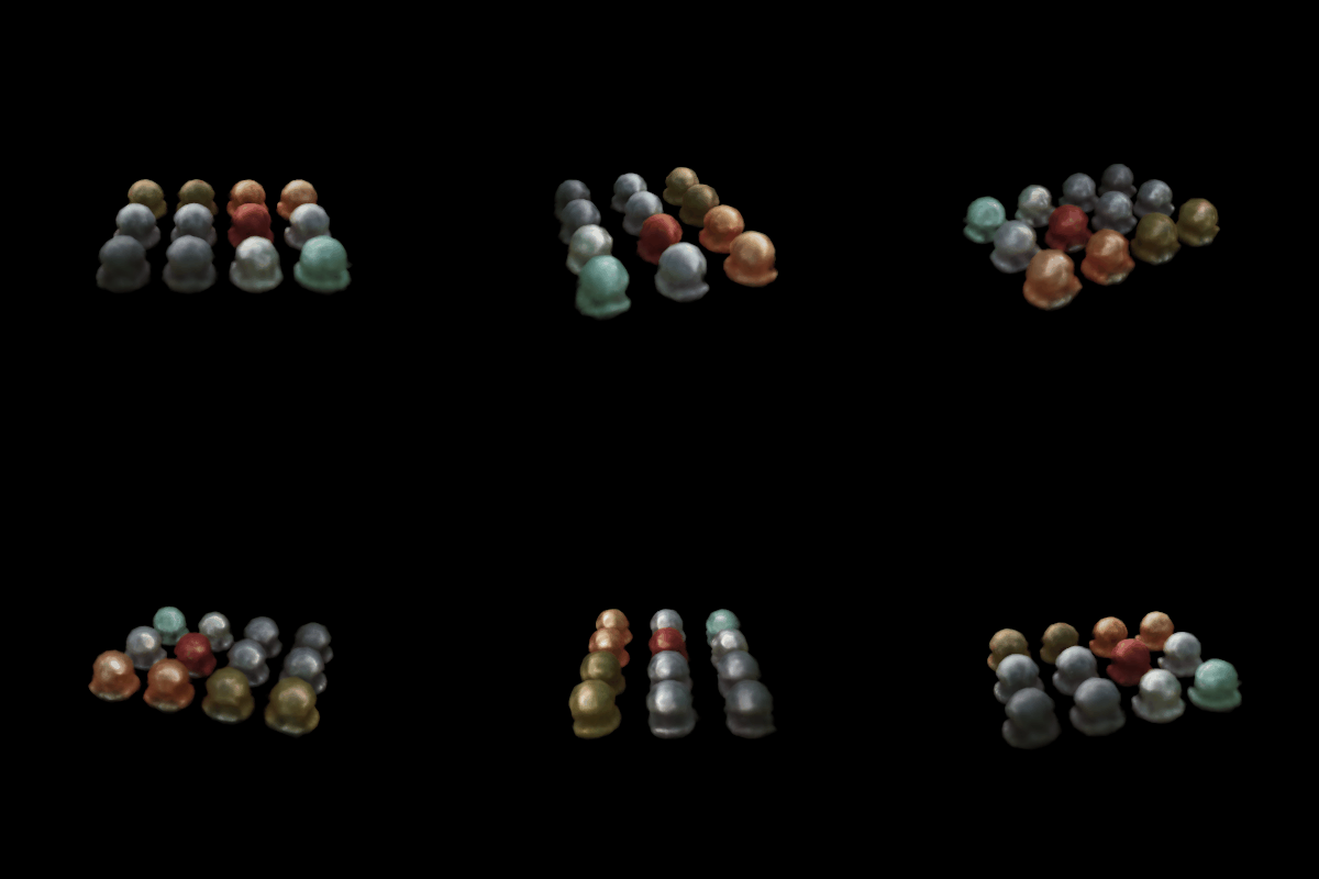
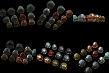
nerf_materials_highres).Trade-off. Adding view dependence improves test PSNR by about 0.4 dB, because the spheres' specular highlights can now move with the camera instead of being averaged into a dull base color. But the train-test gap also grows (0.27 → 0.68 dB), and making the direction branch more expressive (6 frequencies instead of 2) raises train PSNR while slightly lowering test PSNR, with the gap growing to 0.78 dB. That is overfitting: with enough directional capacity, the network can "paint" view-specific colors to match each training image instead of getting geometry and material right, and those painted colors don't carry over to new viewpoints. Keeping density position-only and the direction encoding low-frequency is what keeps that in check.
4.2 Coarse/Fine Sampling 10 bonus
Implement NeRF's coarse/fine strategy: a coarse network estimates geometry, which then guides where the fine network samples. Discuss the speed/quality trade-off.
Two independent NeRF MLPs. The coarse network renders 64 stratified samples per ray. Its
weights (minus the first and last) define a per-ray PDF over depth; I draw 128 extra depths
from it by inverse-transform sampling (torch.searchsorted on the CDF, then
linear interpolation inside the bin). The fine network renders the sorted union of all 192
depths. Both outputs are supervised: loss = MSE(fine) + MSE(coarse).
bins = midpoints(z_coarse)                          # (N, P_c - 1)
pdf  = (w_coarse[:, 1:-1] + 1e-5).normalize()       # detached
cdf  = cat([0, cumsum(pdf)])
u    = rand(N, P_f)                                  # linspace at eval time
idx  = searchsorted(cdf, u, right=True)
z_fine = lerp(bins[idx - 1], bins[idx], (u - cdf[idx - 1]) / (cdf[idx] - cdf[idx - 1]))
z_all = sort(cat([z_coarse, z_fine])) # fine network renders these| Model (lego, 250 epochs) | Network evals per ray | Train time / epoch | Render time / frame | Test PSNR |
|---|---|---|---|---|
| Uniform, 128 samples | 128 | 1.96 s | 156 ms | 24.51 |
| Uniform, 256 samples | 256 | 3.87 s | 540 ms | 24.52 |
| Coarse 64 + fine 128 | 64 + 192 | 3.95 s | 337 ms | 24.74 |
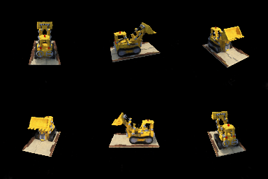
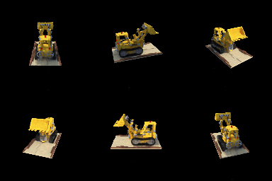
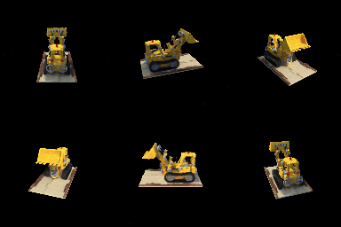
Speed vs. quality. Simply doubling uniform samples from 128 to 256 costs 2× training time and 3.5× rendering time for no gain (+0.01 dB): at 128×128, 128 uniform samples already resolve this scene, and most extra samples land in empty space. At the same number of network evaluations, coarse/fine is the better use of compute (+0.22 dB over 256 uniform), because the fine samples concentrate around surfaces where the coarse weights are high. It also renders faster than 256 uniform, since the coarse pass is cheap. It is still about 2× slower than 128 uniform and has twice the parameters, and the visual difference at this resolution is small; the benefit should grow at higher resolution or with fewer coarse samples, where uniform sampling misses thin surfaces.
4.3 VolSDF 10 bonus
Implement an MLP that predicts signed distance and color (NeuralSurface),
the eikonal loss, and VolSDF's SDF-to-density conversion. Explain what alpha
and beta do, answer the three questions about beta, and comment
on the settings that worked best.
Network. Positional encoding (6 frequencies) → 6-layer, 128-unit
MLPWithInputSkips → a linear distance head with no output
activation (distance can be negative). A 2-layer color MLP with a sigmoid reads the same
features, so get_distance_color shares one forward pass.
# Eikonal: a true SDF has unit-norm gradient everywhere
eikonal_loss = ((gradients.norm(dim=-1) - 1) ** 2).mean()

# VolSDF density: sigma = alpha * Psi_beta(-d), Psi_beta = Laplace CDF (mean 0, scale beta)
half = 0.5 * exp(-|d| / beta)
density = alpha * where(d >= 0, half, 1 - half)
Sphere prior. With a randomly initialized distance network, training
was unreliable: the zero level set starts in random places, so at β = 0.05 training
collapsed with no surface at all, and at β = 0.01 a large spurious "floor" surface
appeared. Following the geometric initialization idea in VolSDF/IDR, I predict distance
as |x| - 1 plus a learned residual, so training starts from a sphere SDF with
the correct sign everywhere. All results below use it.


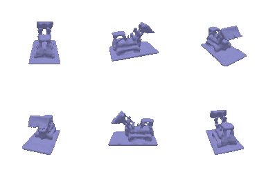
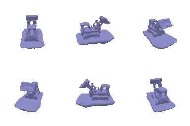
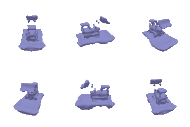
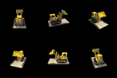
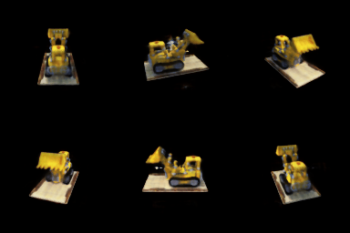
Results (α = 10, eikonal weight 0.02, 128 samples, 250 epochs)
| β | Test PSNR | Geometry |
|---|---|---|
| 0.01 | 21.53 | Sharpest: crisp base-plate edges and bucket |
| 0.05 (default) | 21.53 | Good, slightly rounded edges |
| 0.2 | 20.42 | Blobby, thickened, floating fragments near the arm |
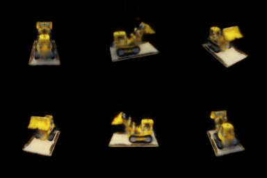
What α and β do
α is the density deep inside the object: Ψ goes to 1 for large negative distance, so density goes to α inside, to 0 outside, and equals α/2 exactly on the surface. It sets how opaque the solid is. β is the scale of the Laplace CDF, i.e. how wide the transition from empty to solid is around the zero level set. Small β makes density a near-step function of the SDF (a hard surface); large β spreads it into a soft shell around the surface.
1. How does high β bias the SDF? Low β?
High β lets the renderer explain the images with a thick, fuzzy shell of density, so the SDF doesn't need its zero level set in exactly the right place. The learned surface comes out smoothed and inflated, and stray density can float near the object, as in the blobby β = 0.2 mesh. Low β makes the rendered images depend almost entirely on where the SDF crosses zero, which biases the SDF toward a tight, sharp surface that sits exactly where the images say it should.
2. Easier to train with low or high β? Why?
High β. Density, and therefore gradient, is nonzero over a wide band around the surface, so many samples along every ray contribute signal even when the current surface is far from correct. With low β, only samples very close to the zero crossing get gradient, so a bad initial surface receives little signal to move. That is why the low-β runs without the sphere prior failed (collapse at 0.05, spurious floor at 0.01), while β = 0.2 still produced a coherent, if blobby, object.
3. More accurate surface with low or high β? Why?
Low β, as long as it trains. Density is concentrated at the zero level set, so the rendering loss directly supervises the surface location instead of a soft average around it. This matches the results: β = 0.01 gives the crispest geometry, with test PSNR equal to β = 0.05 and 1.1 dB better than β = 0.2.
Settings that worked best
β = 0.01 with the sphere prior, α = 10, and eikonal weight 0.02. The sphere prior removes the main disadvantage of low β (fragile early training) by starting from a valid SDF, and then low β gives the sharpest surface. The eikonal term keeps the network an actual distance function, which is what makes the β-controlled transition width meaningful in the first place.
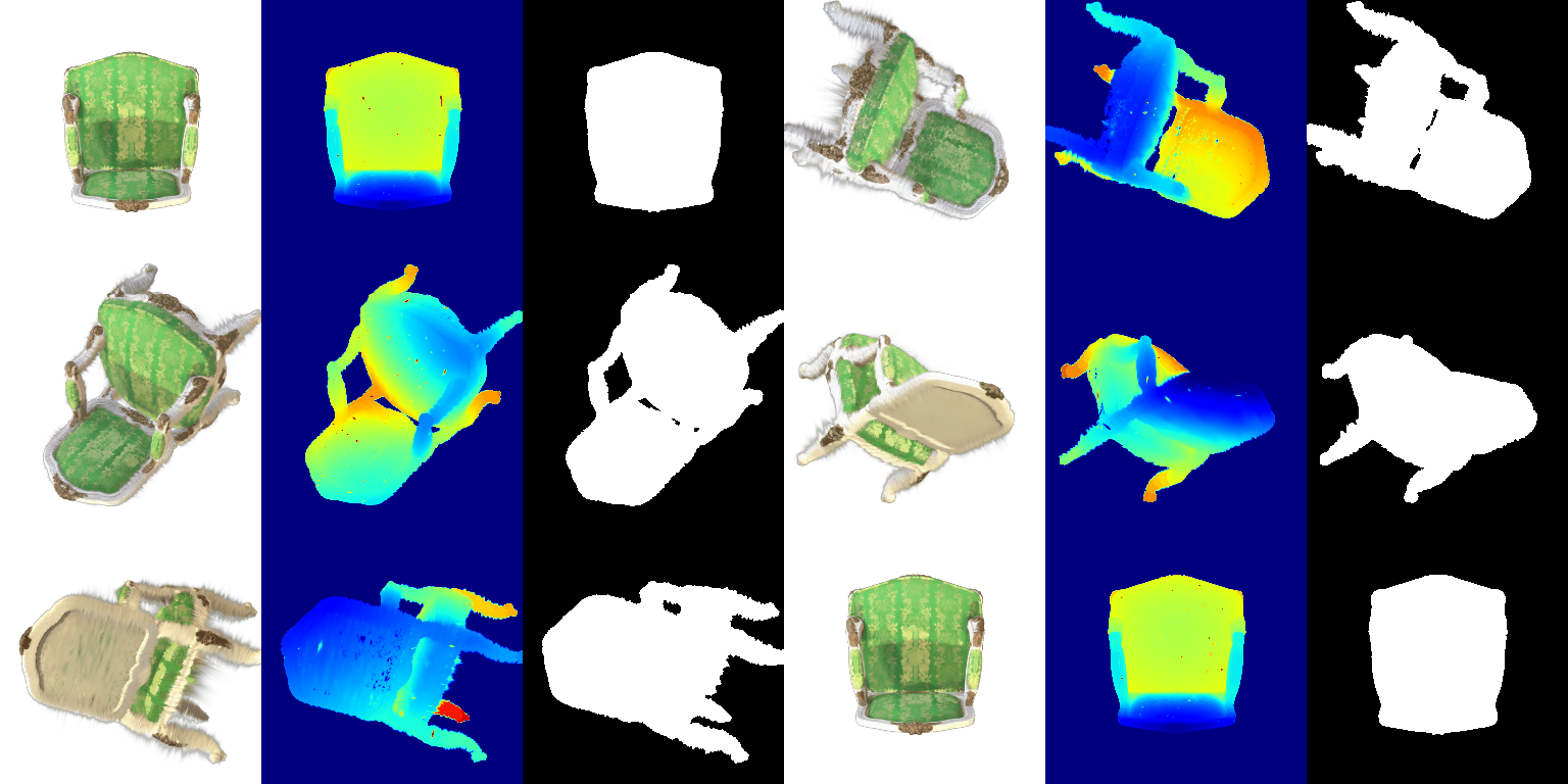
5. 3D Gaussian Rasterization 35 pts
Implement projection of 3D Gaussians to 2D (5.1), 2D Gaussian evaluation (5.2),
depth filtering and sorting (5.3), alpha and transmittance (5.4), and splatting (5.5),
then render the pre-trained chair with render.py.
# 5.1  covariances and projected means
cov_3D = (R * s[:, None, :]) @ (R * s[:, None, :]).T       # R S S^T R^T  (isotropic: s^2 I)
cov_2D = J @ W @ cov_3D @ W.T @ J.T                        # W = camera.R
means_2D = camera.transform_points_screen(means_3D)[:, :2]

# 5.2  exponent of each 2D Gaussian at every pixel
power = -0.5 * einsum('npi,nij,npj->np', x - mu, inv(cov_2D), x - mu)

# 5.3  sort front-to-back, drop Gaussians behind the camera
z = camera.get_world_to_view_transform().transform_points(means)[:, 2]
idxs = argsort(z);  idxs = idxs[z[idxs] >= 0]

# 5.4  alpha and exclusive transmittance
alphas = opacities[:, None] * exp(power)
T = cumprod(cat([T_start, 1 - alphas]), dim=0)[:-1]

# 5.5  composite color, depth, and silhouette with the same weights
w = alphas * T
image = sum(colours * w, 0);  depth = sum(z * w, 0);  mask = sum(w, 0)
The mask is the total accumulated opacity, which is what render uses to
blend in the background color. All four unit tests pass.
6. Training 3D Gaussian Representations 15 pts
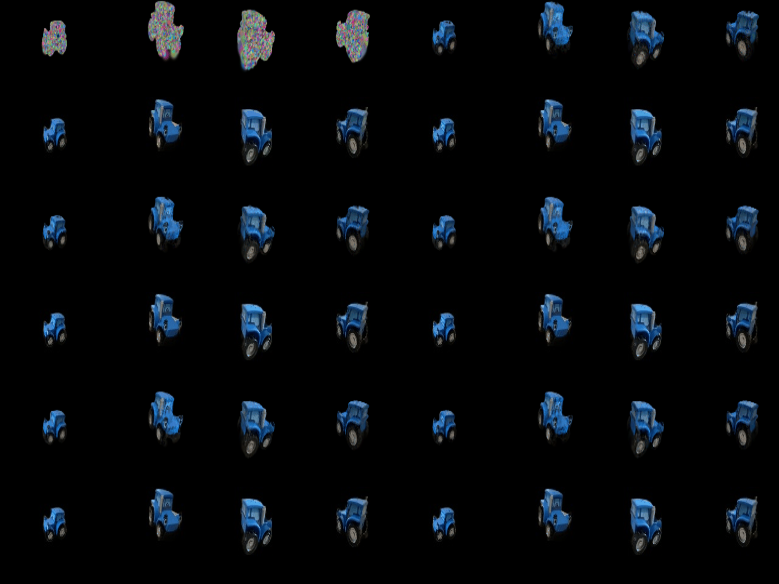
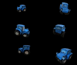
Make the Gaussian parameters trainable, set up the optimizer with per-parameter learning rates, render and compute a loss in the training loop, and train isotropic Gaussians on the toy truck. Report the learning rates, number of iterations, PSNR, SSIM, and both GIFs.
Means, scales, colors, and opacities are trainable (quaternions are unused for isotropic Gaussians). The loss is L1 between the rendered and ground-truth images.
| Parameter | Learning rate |
|---|---|
| Opacities (pre-sigmoid) | 0.05 |
| Scales (log) | 0.005 |
| Colors | 0.01 |
| Means | 0.0005 |
Iterations: 1000. Mean PSNR: 30.010 Mean SSIM: 0.944
Means get the smallest learning rate: the point cloud initialization is already close to the surface, and large position steps scatter the Gaussians. Opacity goes through a sigmoid, so it tolerates a large step size; scales live in log space, where a small step already changes a Gaussian's size noticeably.
7.1 Rendering Using Spherical Harmonics 10 pts
Render the pre-trained chair using all of its spherical harmonic coefficients, attach the GIF next to the 5.5 GIF, and compare 2-3 matching views side by side.
Each Gaussian stores 16 SH coefficients per color channel (degree 3). For the direction from the camera center to each Gaussian, I evaluate the 16 real SH basis functions in one vectorized step and take the weighted sum:
sh = spherical_harmonics.view(N, 16, 3)
dirs = normalize(means_3D - camera.get_camera_center())
basis = stack([C0, -C1*y, C1*z, -C1*x, C2[0]*xy, ..., C3[6]*x*(xx - 3yy)], -1)   # (N, 16)
colours = clamp((basis[..., None] * sh).sum(1) + 0.5, min=0)
As a check, zeroing every coefficient except the DC term reproduces the 5.5 colors exactly.
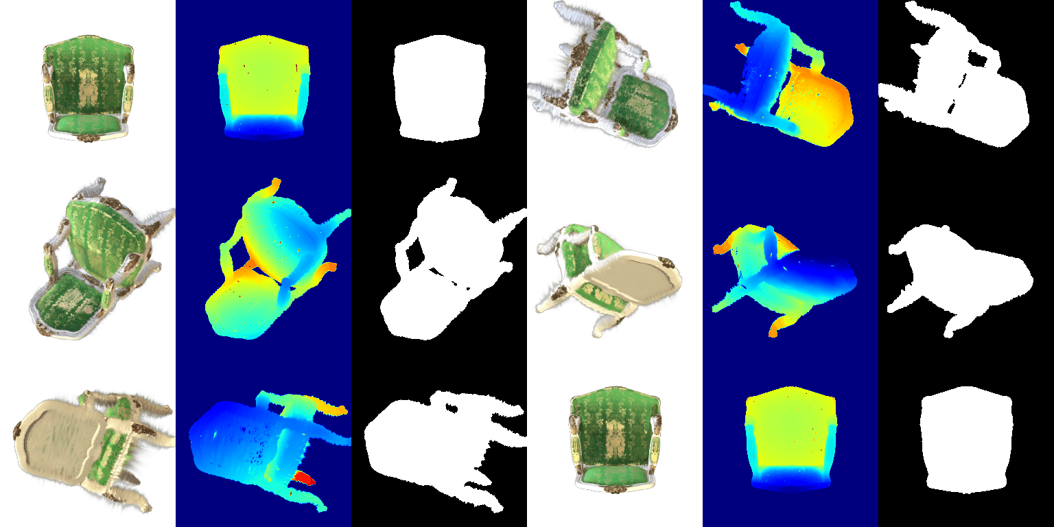
Side-by-side comparisons (left: DC only, right: full SH)


7.2 Training on a Harder Scene 10 pts
Train Gaussians on the NeRF materials scene from random initialization. Compare a baseline using the Q6 setup against an improved approach (GIFs, PSNR, SSIM) and explain every modification.
Baseline: exactly the Q6 setup (same learning rates, L1 loss,
isotropic Gaussians, 1000 iterations) with init_type="random". I then added
improvements one at a time (each row keeps all the changes above it):
| Run | Iterations | PSNR | SSIM |
|---|---|---|---|
| Baseline (Q6 setup) | 1000 | 18.11 | 0.681 |
| + wider, fainter, larger initialization | 1000 | 22.74 | 0.831 |
| + means learning-rate decay | 1000 | 22.78 | 0.832 |
| + L1 + SSIM loss | 1000 | 22.89 | 0.845 |
| + anisotropic Gaussians | 1000 | 23.07 | 0.852 |
| All of the above, trained longer | 5000 | 23.50 | 0.865 |
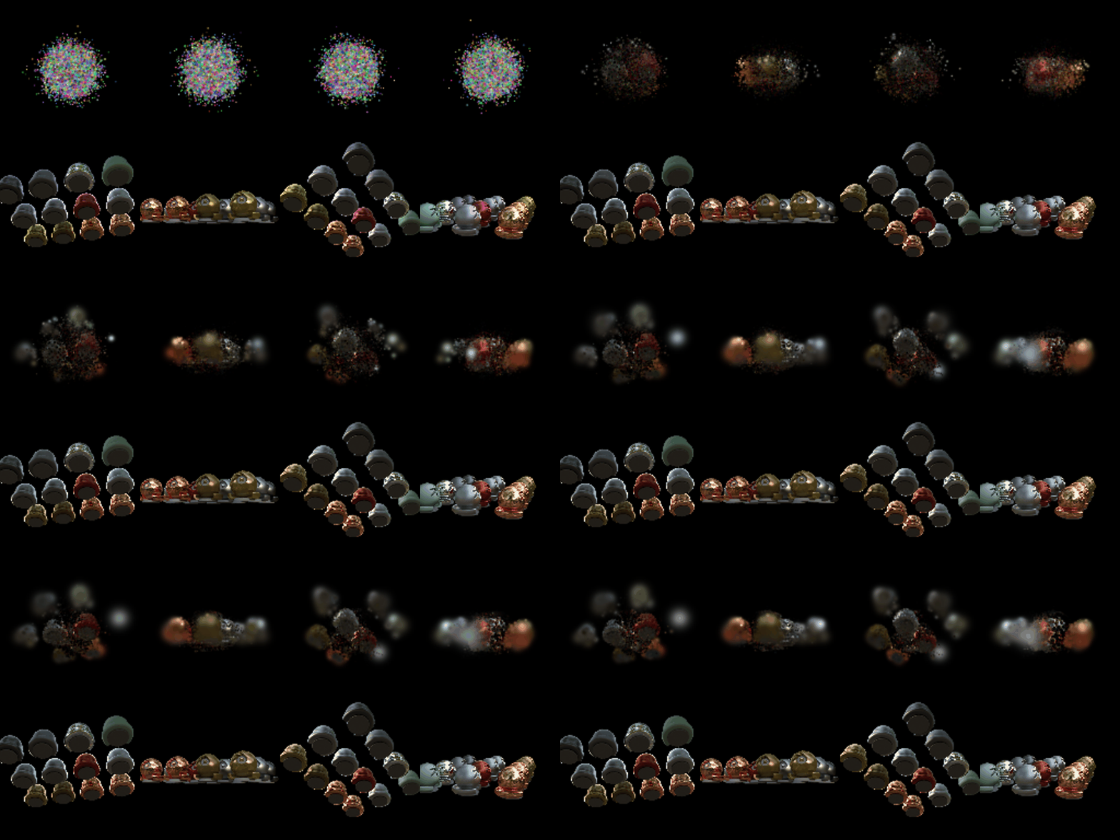
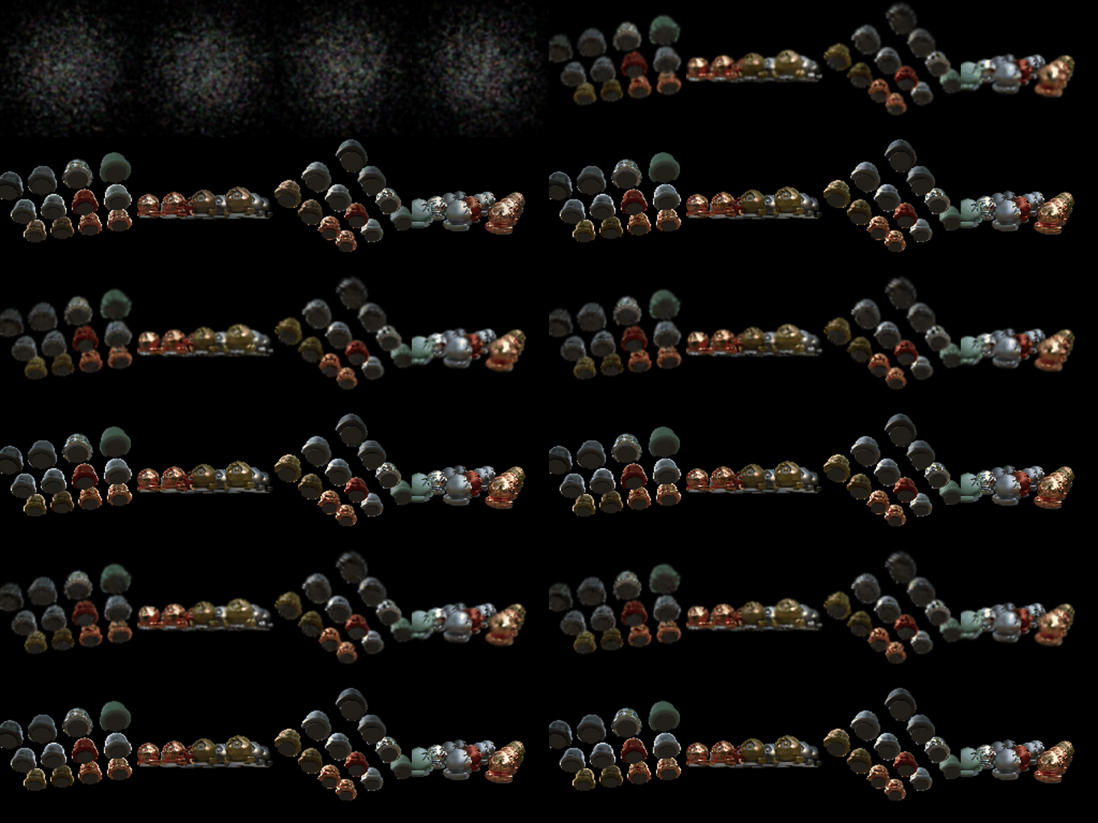

Modifications in the best run
- Initialization (+4.6 dB, by far the largest gain). The cameras sit
4.03 units from the origin with an NDC focal length of 3.125, so the visible region at the
center is about ±1.3 units wide. The default random init (
randn × 0.2) packs every Gaussian within about ±0.4, so spheres away from the center have no Gaussians nearby; in the baseline GIF they never appear. I spread the means with standard deviation 0.7, set initial opacity to 0.1 instead of about 1.0 (fully opaque blobs hide everything behind them and block gradients), and set the initial scale to 0.02 so each Gaussian covers about a pixel at this resolution. - Means learning-rate schedule. 0.002, decaying exponentially to 0.00002 by the last iteration. Random points have to travel far early on, then settle.
- Loss:
0.8 · L1 + 0.2 · (1 − SSIM)(Gaussian window, 11×11, σ = 1.5), as in the 3DGS paper. This mainly helped SSIM (0.832 → 0.845). - Anisotropic Gaussians: per-axis scales plus trainable rotations (quaternion learning rate 0.001), so Gaussians can stretch along the spheres' curved surfaces.
- Longer training: 5000 iterations instead of 1000 (+0.4 dB).
Other learning rates are unchanged from Q6 (opacities 0.05, scales 0.005, colors 0.01). I did not implement adaptive density control; the number of Gaussians stays at 10k.