1.1 Fitting a Voxel Grid 4 pts
Define voxel_loss in losses.py and use it to fit a source
voxel grid directly to a target voxel grid (python fit_data.py --type vox).
Visualize the optimized grid alongside the ground truth.
The voxel decoder everywhere in this assignment outputs unnormalized occupancy logits, so the loss is a sigmoid + binary cross-entropy loss:
def voxel_loss(voxel_src, voxel_tgt):
    loss = F.binary_cross_entropy_with_logits(voxel_src, voxel_tgt)
    return loss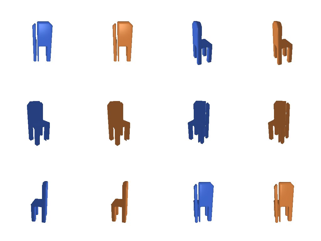
1.2 Fitting a Point Cloud 3 pts
Define chamfer_loss in losses.py (implemented from scratch,
only pytorch3d.ops.knn allowed) and use it to fit a source point cloud to a
target point cloud (python fit_data.py --type point).
For each point in one point cloud, find its nearest neighbor in the other
point cloud via
knn_points and average the squared distances both directions:
def chamfer_loss(point_cloud_src, point_cloud_tgt):
    dist_src = knn_points(point_cloud_src, point_cloud_tgt, K=1).dists[..., 0]
    dist_tgt = knn_points(point_cloud_tgt, point_cloud_src, K=1).dists[..., 0]
    loss_chamfer = dist_src.mean(dim=1) + dist_tgt.mean(dim=1)
    return loss_chamfer.mean()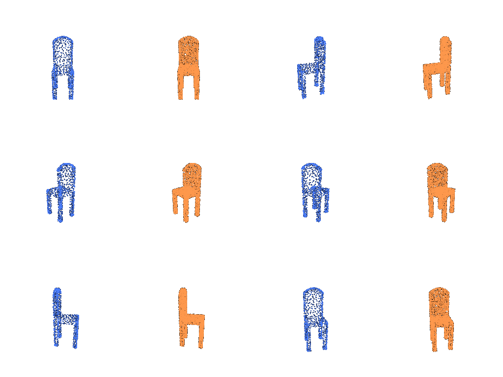
1.3 Fitting a Mesh 3 pts
Define smoothness_loss in losses.py and use it alongside the
chamfer loss to fit a source mesh to a target mesh
(python fit_data.py --type mesh).
Uniform Laplacian smoothing (in starter code): penalize each vertex for deviating from the average position of its neighbors, which means it discourages spiky or folded geometry.
def smoothness_loss(mesh_src):
    loss_laplacian = mesh_laplacian_smoothing(mesh_src, method="uniform")
    return loss_laplacian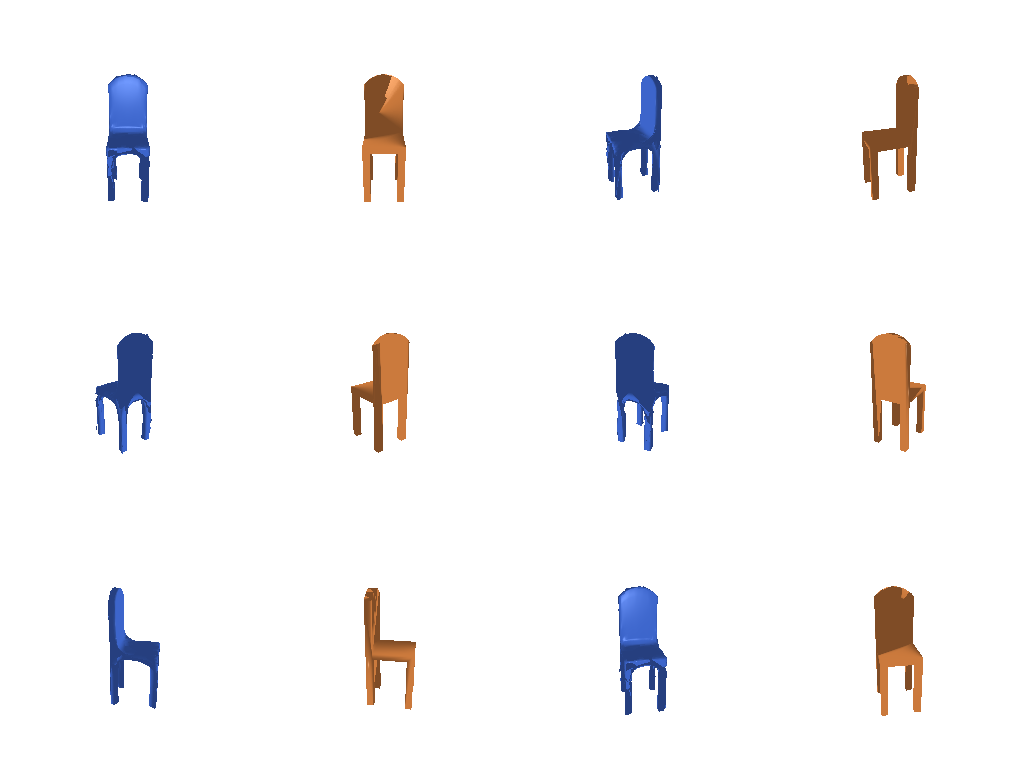
2.1 Image to Voxel Grid 20 pts
Define a decoder network that maps a single-view image feature to a binary voxel
grid, train it (python train_model.py --type vox), then evaluate
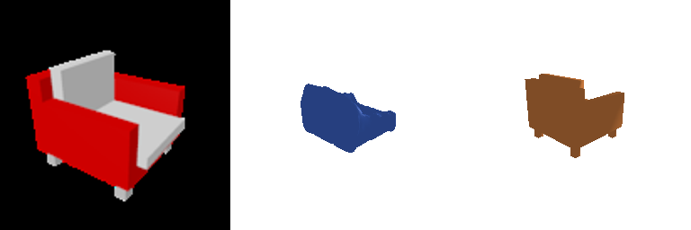
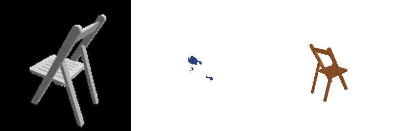
(python eval_model.py --type vox --load_checkpoint). Show 3 test examples
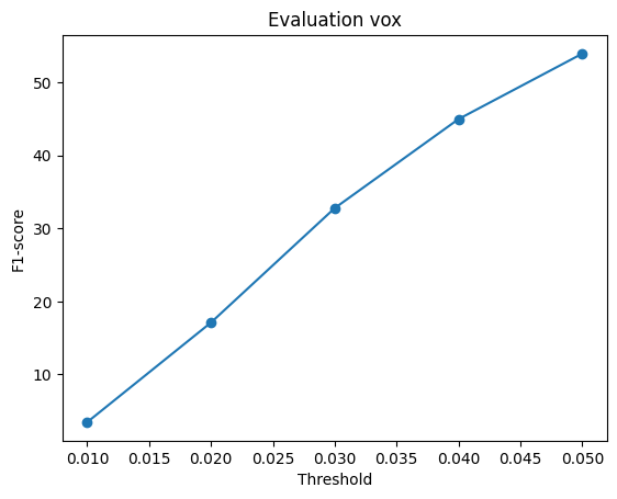
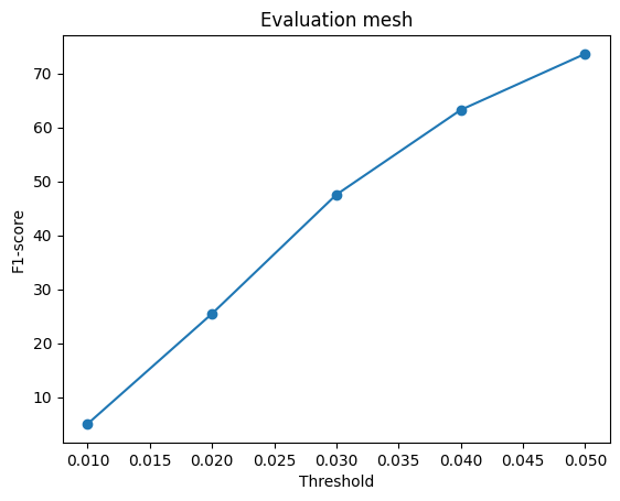
(input RGB, predicted voxel render, GT mesh render) and report F1@0.05 with the F1 plot.
The ResNet-18 image feature (512-d) is reshaped into a 4³ volume and upsampled with
three ConvTranspose3d blocks (stride 2 each) to a 32³ occupancy-logit
grid:
nn.Linear(512, 128*4*4*4) → Unflatten(128,4,4,4)
→ ConvTranspose3d(128,64) → BN → ReLU   # 8³
→ ConvTranspose3d(64,32)  → BN → ReLU   # 16³
→ ConvTranspose3d(32,1)                     # 32³ logits
Avg F1@0.05 = 53.940

2.2 Image to Point Cloud 20 pts
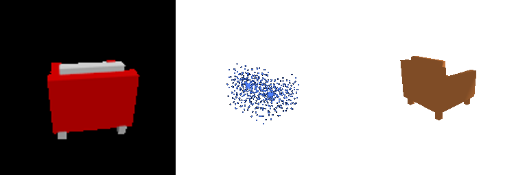
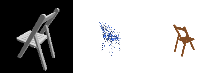
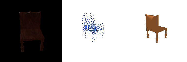
Define a decoder network that maps a single-view image feature to a point cloud, train it, evaluate it, show 3 test examples, and report F1@0.05 with the F1 plot.
A plain MLP regresses all n_points × 3 coordinates directly, squashed
to [-1, 1] with a final Tanh:
nn.Linear(512, 1024) → ReLU
→ nn.Linear(1024, 2048) → ReLU
→ nn.Linear(2048, n_points*3) → Tanh
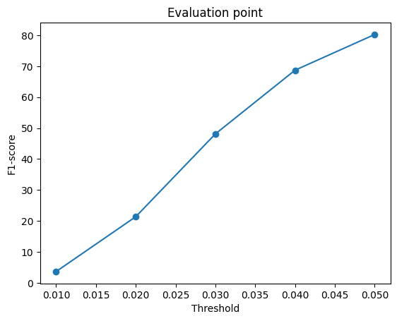
Avg F1@0.05 = 80.220
2.3 Image to Mesh 20 pts
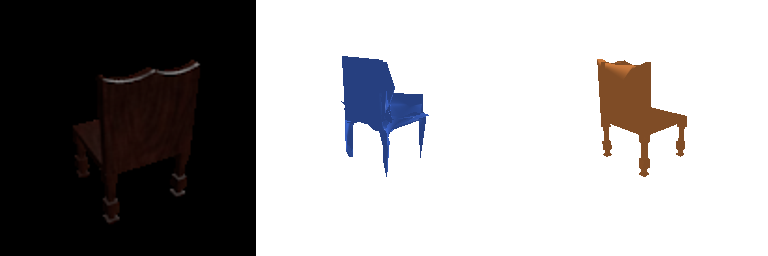
Define a decoder network that maps a single-view image feature to a mesh, train it, evaluate it, show 3 test examples, and report F1@0.05 with the F1 plot. Additionally, quantitatively compare F1 across mesh vs. point cloud vs. voxel grid, with an intuitive explanation.
Starting mesh is an ico-sphere (subdivision level 4, radius 0.4 to roughly match chair scale); the decoder predicts a per-vertex offset and is zero-initialized so training starts from the undeformed sphere:
mesh_pred = ico_sphere(4) scaled by 0.4
nn.Linear(512,1024) → ReLU → nn.Linear(1024,2048) → ReLU → nn.Linear(2048, num_verts*3)
# zero-init the last layer's weight & bias
mesh_pred = mesh_pred.offset_verts(decoder(feat))
Loss combines chamfer distance (on points sampled from both meshes) with the Laplacian
smoothness term from 1.3: loss = w_chamfer * chamfer + w_smooth * smoothness,
with w_smooth = 0.1 here (swept in 2.4).
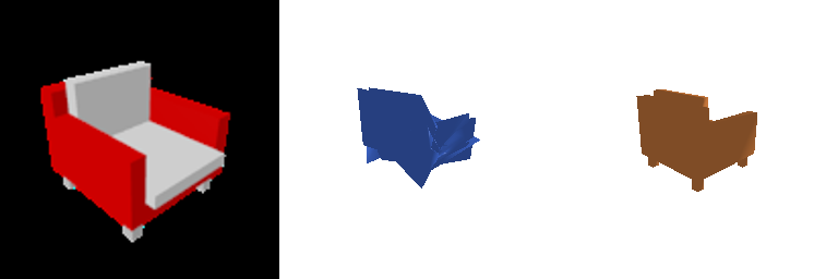
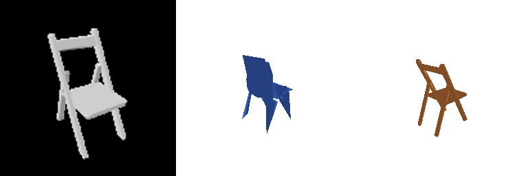
Avg F1@0.05 = 73.642
Comparing mesh vs. point cloud vs. voxel grid
| Representation | F1@0.05 | Why |
|---|---|---|
| Point | 80.2 | Predicts points directly, no lossy conversion step between the network's output and the evaluation metric. |
| Mesh | 73.6 | Spiky/folded surfaces in harder examples (Example 3 above); the ico-sphere start and a modest smoothness weight limit how cleanly it fits thin/concave structure. |
| Voxel | 53.9 | Bounded well below the other two by the representation itself, not just model quality (see below). |
To check whether the voxel gap is a modeling problem or a representation problem, I pushed the ground-truth voxel grid through the exact same evaluation pipeline (marching cubes → sample points → frame alignment) and scored it against its own ground-truth mesh. Even a perfect voxel prediction only reaches 76.5 F1@0.05, while our trained model's 53.9 is about 70% of that ceiling, not 70% of 100. Comparing predicted vs. ground-truth mesh bounding boxes shows why: voxelized shapes come out roughly 13% wider in x/z and 3% taller in y, consistent with the reconstructed surface sitting about one voxel (≈0.03 in normalized units) outside the true surface. At 32³ resolution, thin parts like chair legs and backs get fattened by a voxel's worth of margin on every side. So part of the voxel grid's F1 deficit is a hard limit of 32³ discretization combined with this evaluation protocol, not purely a weaker decoder.
Note on the 53.9 number itself: this run used the
full image encoder end-to-end (not the precomputed --load_feat features) for the same 10,000-iteration,
batch-32 budget as point and mesh above, so the gap isn't a training-shortcut artifact. The
76.5 ceiling measurement above is the explanation this training setup supports.
2.4 Analyze Effects of Hyperparameter Variation 10 pts
Vary a hyperparameter of your choice and analyze the results.
I swept the mesh smoothness weight w_smooth ∈ {0, 0.01, 0.1, 1, 5}
(chamfer weight fixed at 1.0, same training budget as 2.3), on the same test chair:
| w_smooth | 0 | 0.01 | 0.1 | 1 | 5 |
|---|---|---|---|---|---|
| F1@0.05 | 74.80 | 75.33 | 73.64 | 71.36 | 64.22 |
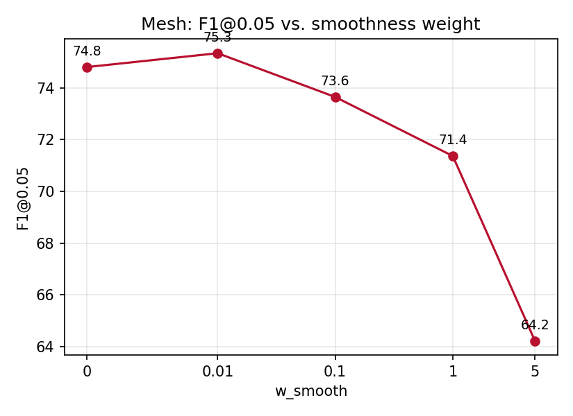
w_smooth (log-ish x-axis).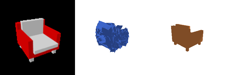
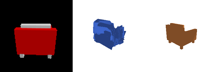
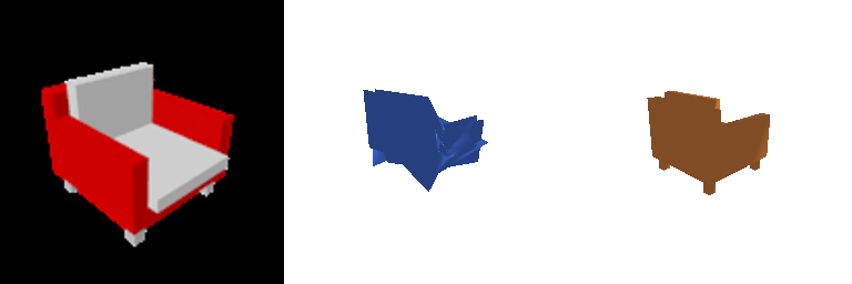
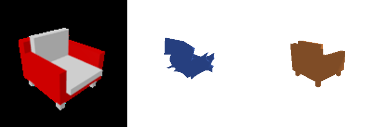
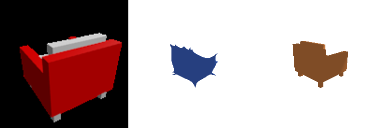
F1 peaks at a small but nonzero smoothness weight (0.01) and stays close to that at 0 and
0.1, then drops sharply once smoothing dominates (1, 5). This matches the renders: at
w_smooth=0 the chamfer term alone leaves the mesh spiky and self-intersecting,
which is locally wrong but still close to the target surface on average, so F1 isn't badly
hurt. As w_smooth grows, the Laplacian term increasingly wins the trade-off
against chamfer accuracy, visibly rounding off the chair's arms and back and pulling the
surface away from the true shape. At w_smooth=5 the prediction is a
smooth blob with most chair-specific structure gone, and F1 score thus falls off. A little
smoothing cleans up the bad spiky behavior, but too much suppresses shape accuracy in
exchange for a nicer-looking (but wronger) surface.
2.5 Interpret Your Model 10 pts
Create visualizations that help highlight what the learned model does, beyond final predictions and numbers.
Per-vertex error heatmaps
For 5 test examples per representation, I color each predicted vertex by its nearest-neighbor distance to the ground-truth surface (green = low error, red = high error):

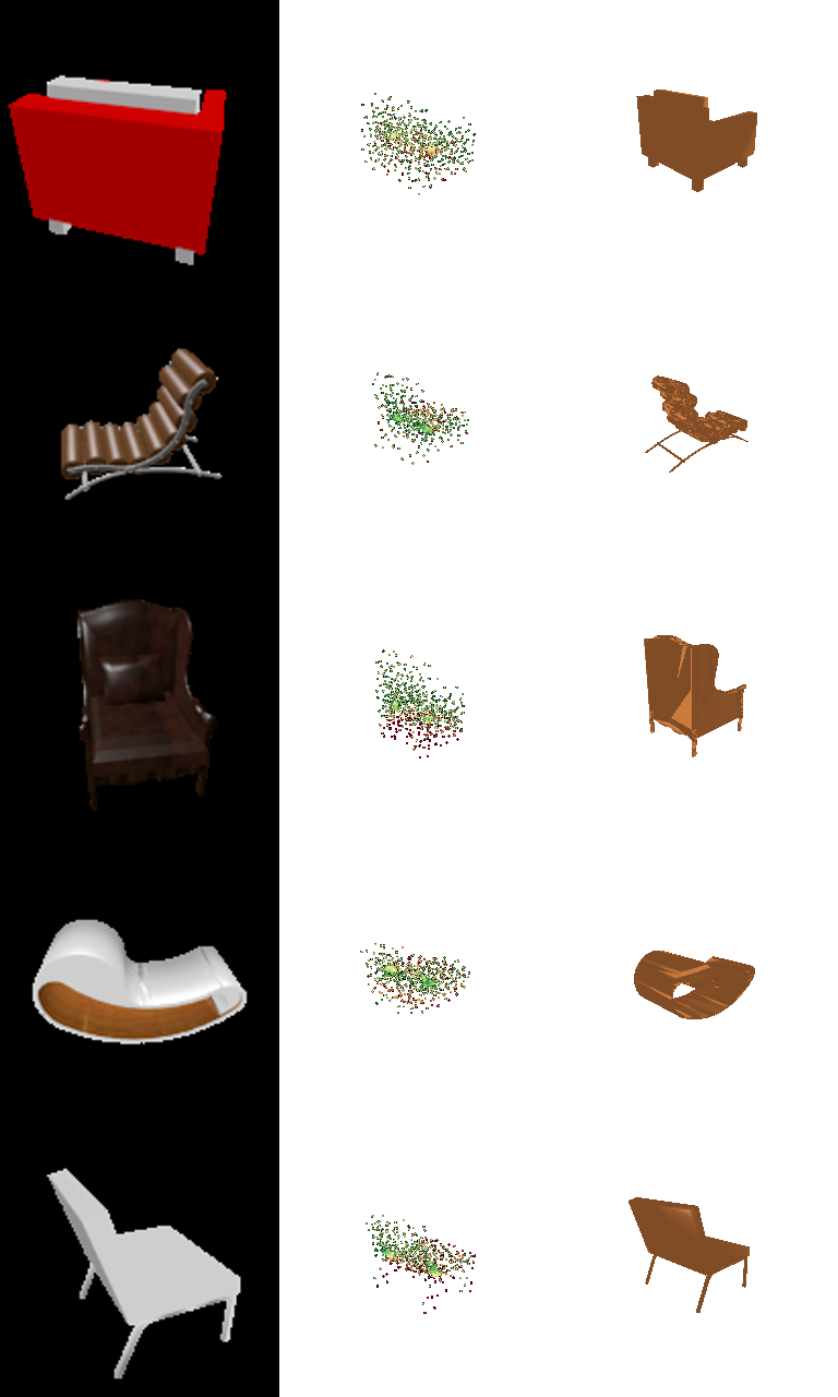
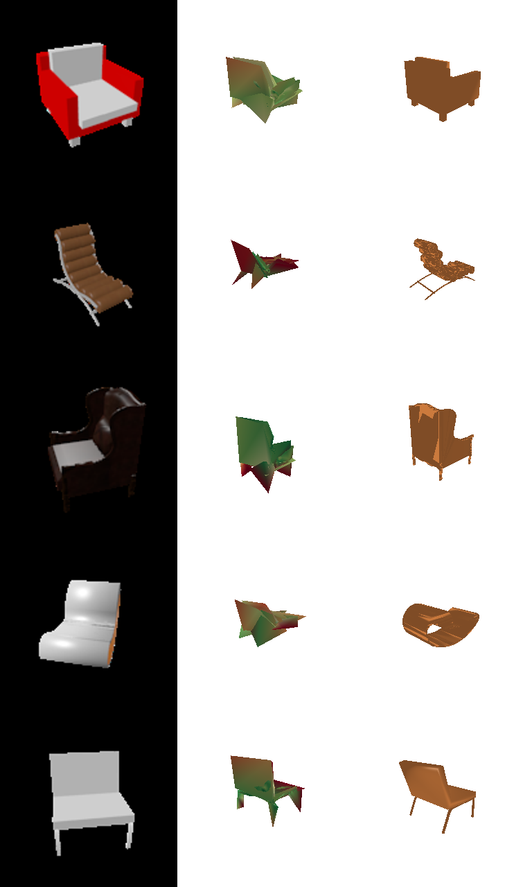
The mesh grid's row 2 and 4 are failure cases worth discussing: in both cases the ground-truth chair is an "unusual" shape while the prediction collapses to a generic "chair" shape from the dataset. This is the "average shape" behavior: when a single global image feature under-constrains the decoder, it's cheaper for training to regress toward the dataset's modal chair shape than to commit to an unusual one, and most of these errors (red regions) sit exactly on the atypical parts of the geometry.
Diversity: predictions vs. ground truth
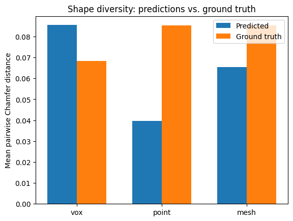
To check that "average shape" intuition directly, I measured mean pairwise Chamfer distance among 60 predicted shapes vs. among their 60 ground-truth counterparts, per representation: a proxy for how varied the outputs are, independent of how accurate any single one is:
| Type | Pred. diversity | GT diversity | Ratio |
|---|---|---|---|
| Point | 0.040 | 0.085 | 0.46 |
| Mesh | 0.065 | 0.085 | 0.77 |
| Vox | 0.085 | 0.068 | 1.25 |
Point-cloud predictions are the least diverse relative to the real spread of the data (ratio 0.46), the strongest quantitative evidence of average-shape collapse, and consistent with it scoring highest on F1 while still being the model most prone to settling on a generic chair shape instead of the exact instance. Mesh is closer to the true spread (0.77). Voxel is actually more varied than the ground truth (1.25), but based on examples like the thin folding chair in 2.1, this looks less like genuine shape diversity and more like noisy, fragmented marching-cubes surfaces inflating the pairwise distances.
3.1 Implicit Network 10 pts
Implement an implicit decoder that takes 3D locations as input and outputs an
occupancy value, conditioned on the image feature. Query a 32×32×32 meshgrid
in the normalized coordinate space (-1,1)³ to produce the full occupancy
output.
An MLP takes the concatenation of the 512-d image feature and a 3D query coordinate and
outputs one occupancy logit. It's queried on all 32,768 cells of a dense grid spanning
(-1,1)³ every forward pass (no subsampling), ordered to match the existing
voxel ground-truth layout, so the output is a drop-in 32³ logit
volume that reuses the exact same BCE loss, marching-cubes evaluation, and visualization
code as 2.1. The query coordinate is NeRF-style positional-encoded (6 frequency bands of
sin/cos) before being concatenated with the image feature, since a raw (x,y,z)
input makes it hard for a plain MLP to represent the high-frequency occupancy boundaries
of a 32³ grid:
pe(xyz) = concat(xyz, sin(2^k π xyz), cos(2^k π xyz) for k=0..5)   # 3 -> 39 dims
feat (B,512) + pe(xyz) (N,39), N = 32³, broadcast → (B,N,551)
nn.Linear(551,512) → ReLU → nn.Linear(512,512) → ReLU
→ nn.Linear(512,256) → ReLU → nn.Linear(256,1)   # occupancy logit per query point
→ reshape to (B,1,32,32,32)
Avg F1@0.05 = 49.649 (Precision 68.6, Recall 45.5); similar to the conv-decoder voxel baseline (53.9). An earlier version — no positional encoding, and trained at half the batch size of every other model on this page — scored only 31.7 (Precision 68.3, Recall 26.3); fixing both raised it to the number above.
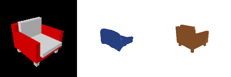
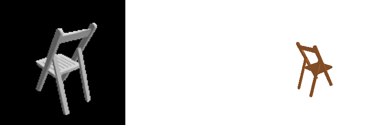
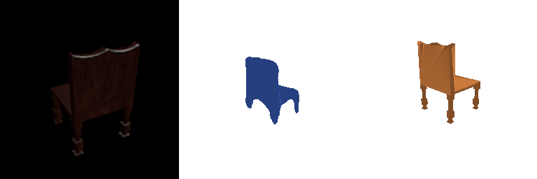
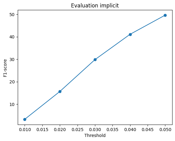
Precision barely moved (68.3 → 68.6) while recall nearly doubled (26.3 → 45.5): the model was never predicting garbage, it was under-predicting, and both fixes attacked exactly that. Example 3 shows it clearly: the same ornate chair that used to come out as a disconnected fragment is now one solid, recognizably chair-shaped blob. But Example 2, the thin folding chair, is still a complete failure (empty prediction): its legs and back are only 1–2 voxels thick at 32³ resolution, and with a single global image feature and no local/multi-resolution conditioning, the decoder still can't resolve structure that fine. That residual gap is exactly the kind of limitation convolutional / local-feature follow-ups to occupancy networks (referenced in the handout) are built to address, and is consistent with this being a genuine representational ceiling rather than an artifact of how it was trained.
3.2 Parametric Network 10 pts
Implement a parametric function that takes sampled 2D points as input and outputs their corresponding 3D points.
AtlasNet-style decoder: the point budget is split across num_patches = 4
small MLPs, each owning its own 2D patch. Every patch MLP takes the 512-d image feature
concatenated with a randomly-sampled 2D point in [-1,1]² and maps it to
an xyz coordinate; the four patches' outputs are concatenated into one point
cloud, so this reuses the chamfer loss and point-cloud evaluation/visualization from 2.2
unchanged:
# per patch p = 1..4:
uv ~ Uniform([-1,1]²),  feat (B,512) broadcast → (B, pts_per_patch, 514)
nn.Linear(514,256) → ReLU → nn.Linear(256,256) → ReLU
→ nn.Linear(256,128) → ReLU → nn.Linear(128,3) → Tanh
# concat all 4 patches' points -> (B, n_points, 3)
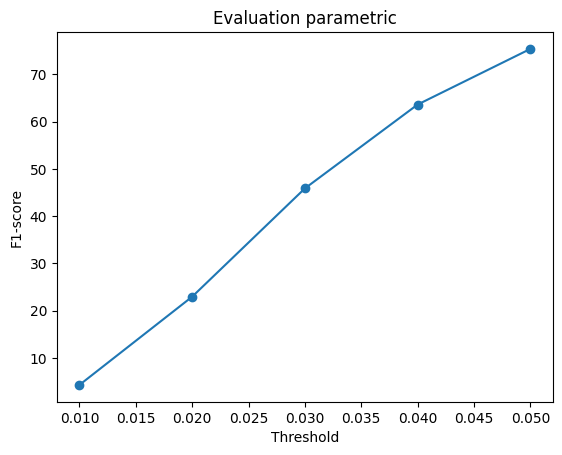
Avg F1@0.05 = 75.353 (Precision 77.4, Recall 74.5), right in the range of the point (80.2) and mesh (73.6) baselines, far ahead of both voxel (53.9) and the implicit decoder (49.6) above.
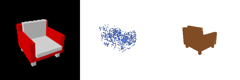
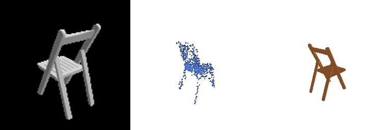
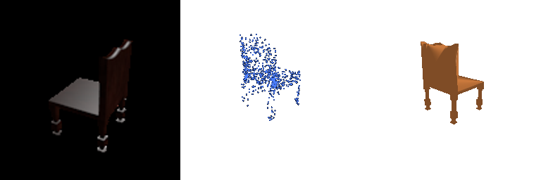
Unlike the implicit decoder, the parametric network handles thin structure well (Example 2's folding-chair legs are clearly recovered): each patch only has to learn a local 2D-to-3D deformation rather than a global occupancy function over the whole volume, and directly regressing xyz sidesteps both the 32³ discretization limit that caps voxel/implicit performance (2.3) and the all-or-nothing nature of occupancy classification.
Summary: All Five Representations
| Type | F1@0.05 | Precision@0.05 | Recall@0.05 |
|---|---|---|---|
| Point (2.2) | 80.2 | — | — |
| Parametric / AtlasNet (3.2) | 75.4 | 77.4 | 74.5 |
| Mesh (2.3) | 73.6 | — | — |
| Voxel (2.1) | 53.9 | — | — |
| Implicit (3.1) | 49.6 | 68.6 | 45.5 |
Decoders that regress coordinates directly (point, parametric) win on this metric; decoders built on an intermediate 32³ occupancy grid (voxel, implicit) are capped by the resolution/discretization ceiling derived in 2.3. The implicit network needed a positional encoding on its query coordinate just to get close to the conv-decoder voxel baseline it's conceptually equivalent to (3.1). Even then, both still fail outright on thin structure (the folding chair in 2.1/3.1) that point/parametric recover without difficulty, since coordinate regression isn't bottlenecked by a fixed voxel grid. The mesh decoder sits in between: coordinate regression like point/parametric, but constrained by a fixed topology (ico-sphere) and a smoothness/accuracy trade-off (2.4) that a free-form point cloud doesn't have to make.