Assignment 3
1. Differentiable volume rendering
1.3 Ray sampling


1.4 Point sampling

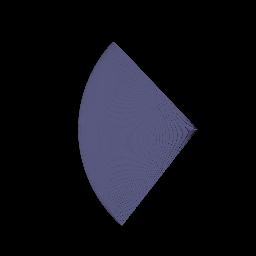
1.5 Volume rendering


2. Optimizing a basic implicit volume
| x | y | z | |
|---|---|---|---|
| Box center | 0.25 | 0.25 | 0.00 |
| Box side lengths | 2.01 | 1.50 | 1.50 |


3. Neural Radiance Field


Validation PSNR: 23.82 dB
4. NeRF extras
4.1 View dependence (materials)
Density depends on position only; color also takes the encoded view direction.


| Val PSNR | |
|---|---|
| No view dependence | 24.10 dB |
| View dependence | 25.03 dB |
- Gain: +0.9 dB; highlights and reflections on the shiny spheres are modeled.
- Cost: more parameters. With few training views, the color branch can explain the training images without the right geometry, which hurts novel views.
4.2 Coarse / fine sampling (lego)
64 coarse samples, then 64 extra samples drawn from the coarse weights; the fine network renders the merged 128 points. Loss = coarse MSE + fine MSE.

| Single net | Coarse + fine | |
|---|---|---|
| Val PSNR | 23.82 dB | 24.02 dB |
| Render one 128×128 image | 88 ms | 228 ms (2.6×) |
| Parameters | 93 k | 186 k |
- Quality: +0.2 dB.
- Speed: 2.6× slower rendering and twice the parameters.
4.3 VolSDF (lego)
Density = α · Ψβ(−d), with Ψβ the CDF of a zero-mean Laplace distribution. Loss = color MSE + 0.02 · eikonal.


What α and β do
- α is the density inside the object, i.e. how opaque it is. Large α stops a ray at the surface; small α gives a translucent object.
- β is the width of the transition at the surface. Small β gives a near-step density (sharp surface); large β gives a smooth, blurry transition. At
d = 0the density isα/2.
Varying β
Top row: geometry. Bottom row: color.


| β | Val PSNR | Geometry |
|---|---|---|
| 0.01 | 21.47 dB | sharpest; cab pillars and base detail kept |
| 0.05 | 21.27 dB | good, slightly smoother |
| 0.5 | 18.48 dB | blobby; thin structures lost |
Best setting: α = 10, β = 0.01, eikonal weight 0.02, sphere initialization of the SDF (radius 1).
Questions
- How does β bias the SDF? High β spreads the density over a wide band around the surface, so the zero level set is not pinned down: the SDF becomes smooth and rounded and details wash out. Low β makes the density an almost sharp step at the surface, which keeps details.
- Easier to train: low or high β? In principle high β: density is non-zero far from the surface, so rays give gradients that can move the surface. With low β only samples inside the thin band give signal. In my runs all three trained, because the sphere initialization already put the surface close.
- Accurate surface: low or high β? Low β: density concentrates at the zero level set, so the extracted mesh is sharper and more faithful (best at β = 0.01, worst at β = 0.5).
5. 3D Gaussian rasterization

6. Training 3D Gaussians
| Setting | Value |
|---|---|
| Learning rates | opacities 0.05 · colours 0.02 · scales 0.005 · means 0.0005 |
| Iterations | 1000 |
| Test PSNR / SSIM | 29.25 dB / 0.939 |


7. Extensions
7.1 Spherical harmonics

Same view, left: without SH, right: with SH.


- Color depth: with SH the greens are deeper and more saturated; without SH the image looks washed out.
- Texture: the golden brocade pattern is sharp and high-contrast with SH, and smeared without it.
- Shading: the backrest has a blurry dark patch without SH; with SH the shading follows the surface and the viewing angle.
7.2 Training on a harder scene
Materials scene, random point initialization (no clean point cloud to start from).


| PSNR | SSIM | |
|---|---|---|
| Baseline (6.2 recipe, isotropic, random init) | 18.411 dB | 0.676 |
| Improved | 19.740 dB | 0.746 |
Changes in the improved recipe (vs. 6.2):
- Anisotropic Gaussians instead of isotropic, so each Gaussian can stretch along the directions it actually needs to cover the surface instead of being a blurry sphere.
- Wider / larger initialization (mean std 0.2 → 0.5, max scale 0.01 → 0.03) so the randomly-placed Gaussians have more initial spread and overlap to converge from, instead of starting as a tight, mostly-empty cluster at the origin.
- Exponential learning-rate decay on all parameters (down to 10% of the initial value by the last iteration), for coarse-to-fine convergence instead of a constant step size.
- SSIM loss term (weight 0.2) added to the per-pixel colour loss, which pushes on structural/contrast similarity rather than raw pixel error alone.
- Adaptive density control (relocation): starting at iteration 200 and every 100 iterations after, Gaussians with opacity below a threshold are relocated to higher-opacity regions, so capacity gets moved to where the scene actually needs it instead of being wasted on near-transparent points.
Together these give +1.33 dB PSNR and +0.07 SSIM over the baseline on this harder, randomly-initialized multi-object scene.