Assignment 2
Question 1: Exploring loss functions
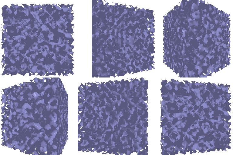
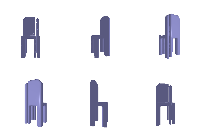
1.1: Fitting a voxel grid
| Starting voxel grid | Ground truth voxel grid | Optimized voxel grid |
|---|---|---|
 |
 |
 |
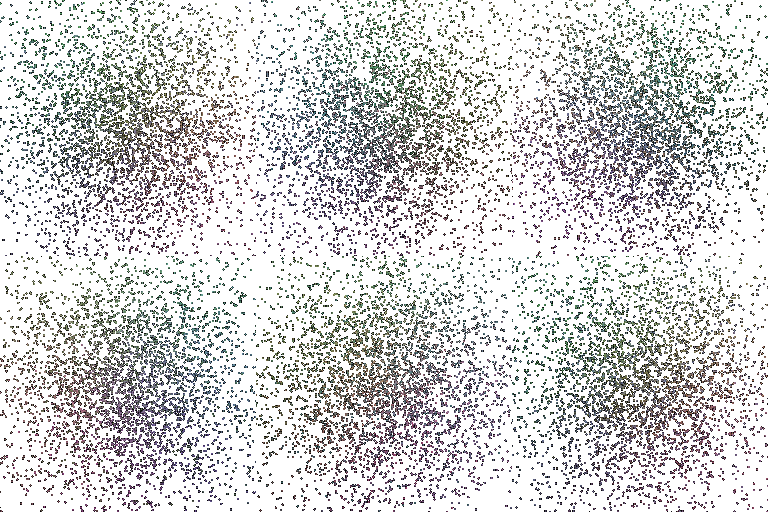
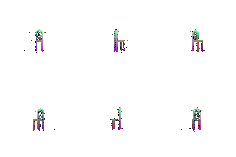
1.2: Fitting a point cloud
| Starting point cloud | Ground truth point cloud | Optimized point cloud |
|---|---|---|
 |
 |
 |
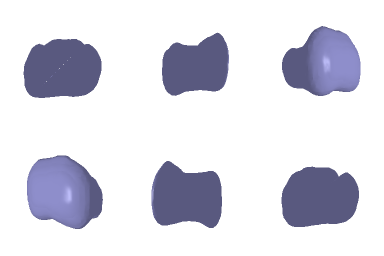
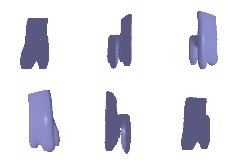
1.3: Fitting a mesh
| Starting mesh | Ground truth mesh | Optimized mesh |
|---|---|---|
 |
 |
 |
Question 2: Reconstructing 3D from single view
This assignment submission used the
--load_featargument to use pretrained ResNet18 features.
2.1: Image to voxel grid
| Input RGB | Ground truth | Predicted |
|---|---|---|
 |
 |
 |
 |
 |
 |
 |
 |
 |
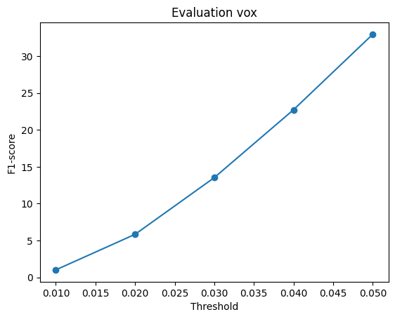
Avg F1@0.05: 32.979
F1 score plot:
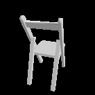
2.2: Image to point cloud
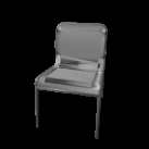
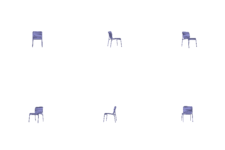
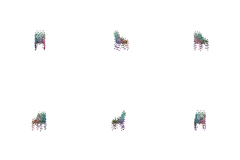
| Input RGB | Ground truth | Predicted |
|---|---|---|
 |
 |
 |
 |
 |
 |
 |
 |
 |
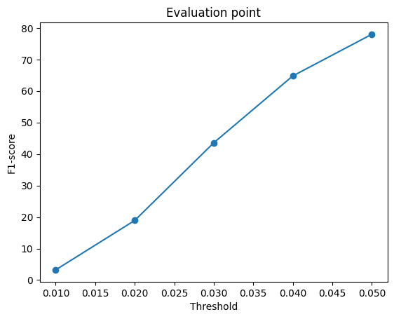
Avg F1@0.05: 77.984
F1 score plot:
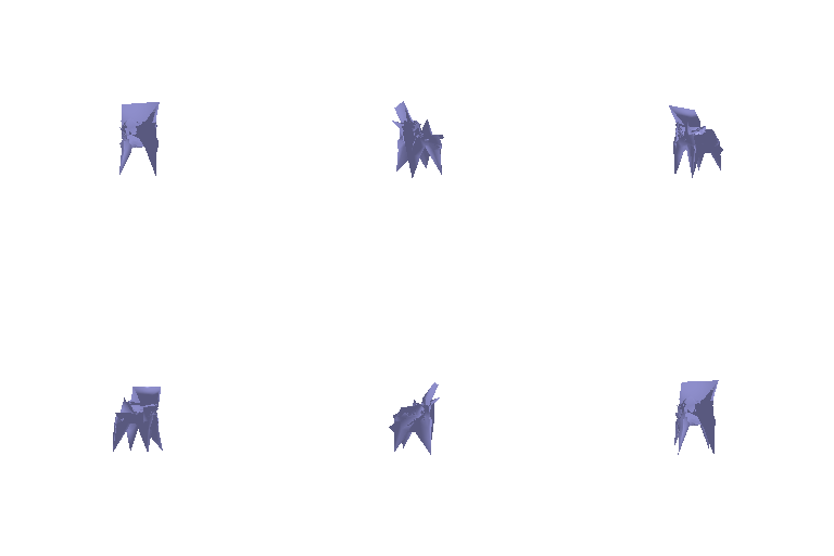
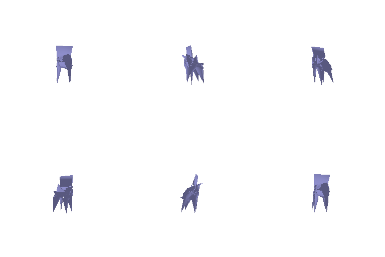
2.3: Image to mesh
| Input RGB | Ground truth | Predicted |
|---|---|---|
 |
 |
 |
 |
 |
 |
 |
 |
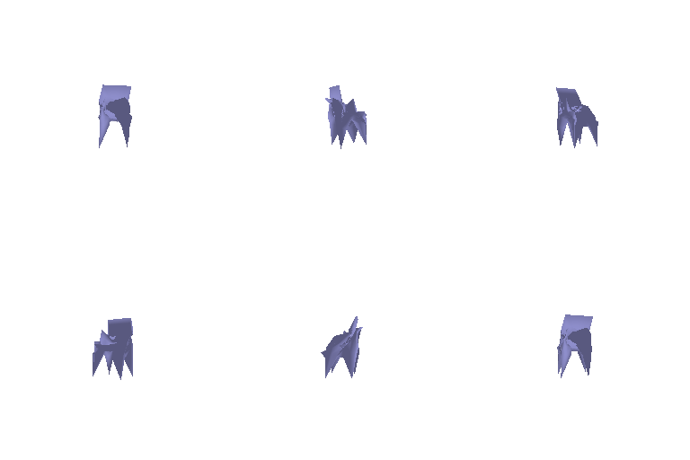 |
Avg F1@0.05: 48.653
F1 score plot:
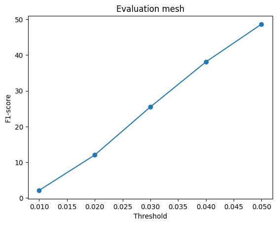
F1 score comparision
| Voxel grid F1 plot | Point cloud F1 plot | Mesh F1 plot |
|---|---|---|
|
|
|
The F1 scores for point clouds is maximum followed by the mesh predictions and then the voxel predictions.
One reason for F1 score being low for voxel predictions is that the voxel output goes through marching cubes before being sampled for metric calculation but the voxel network optimizes BCE classification per voxel which does not directly help with optimizing the surface geometry.
Since the point cloud loss directly optimizes chamfer distance which is what the F1 score directly measures, the F1 score is highest among the three.
The mesh loss combines a sampled chamfer distance along with a laplacian smoothing loss which does not directly optimize for the F1 score, hence the score is between the two.
2.4: Analyse effects of hyperparams variations
I changed the w_smooth parameter for the 2D image to 3D mesh. I used w_smooth = 0.5 for my regular training and explored w_smooth = 0.1 and w_smooth = 0.9:
| w_smooth=0.1 | w_smooth=0.5 | w_smooth=0.9 |
|---|---|---|
 |
|
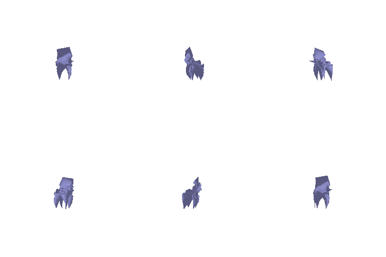 |
The output predictably shows a sharp pointier output with self intersections and jagged surface when the smoothing factor is low and a rounded geometry when the smoothing factor is higher. It can be predicted that an even higher smoothing factor would push the output more towards the initialized sphere mesh.
2.5: Interpret your model
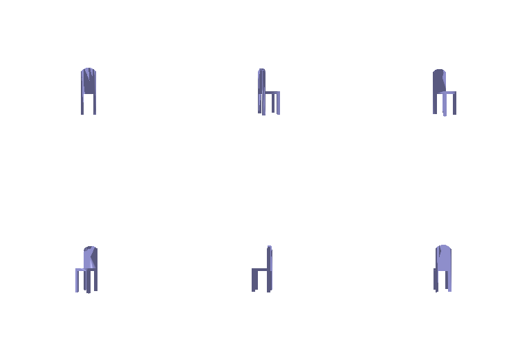
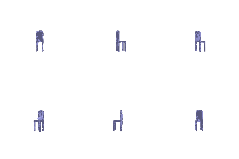
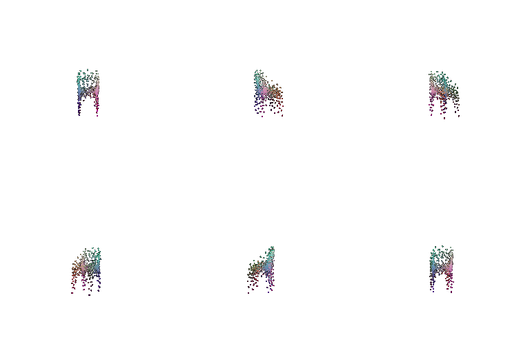
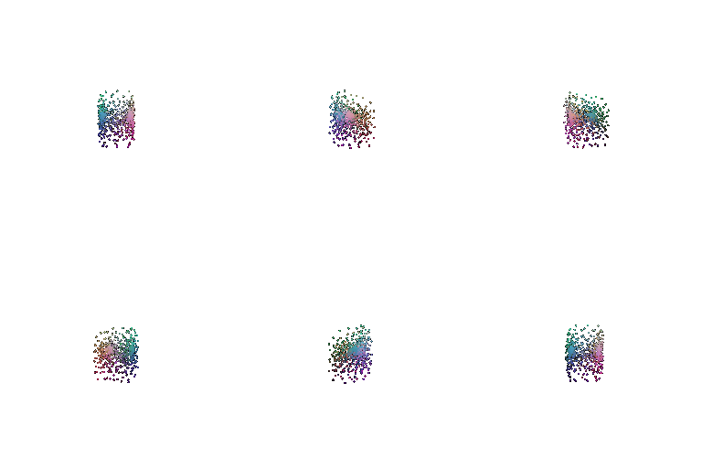
I chose to perform a visualization that shows the implicit field predicted for a few samples across XY, XZ, and YZ planes:
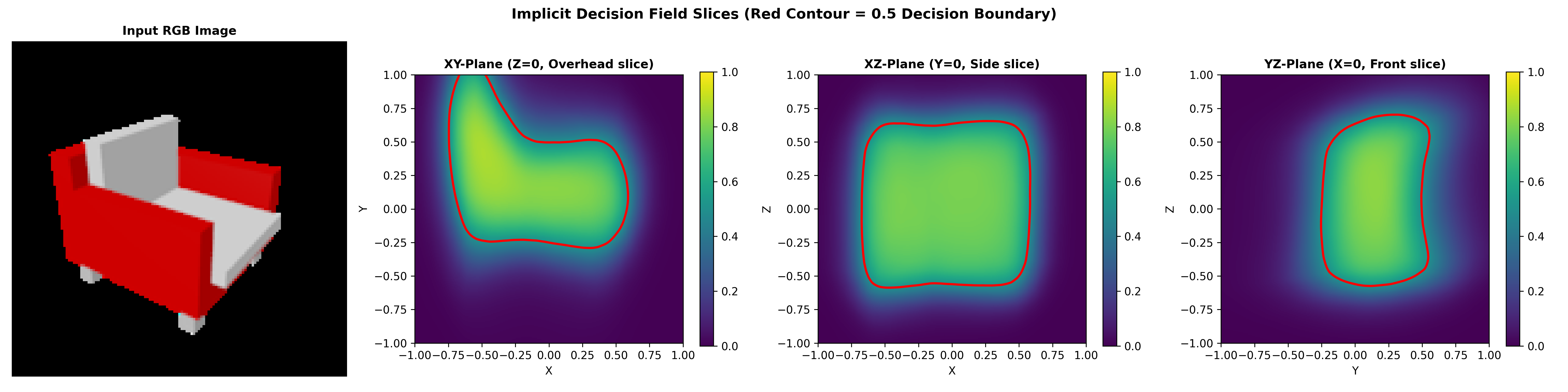
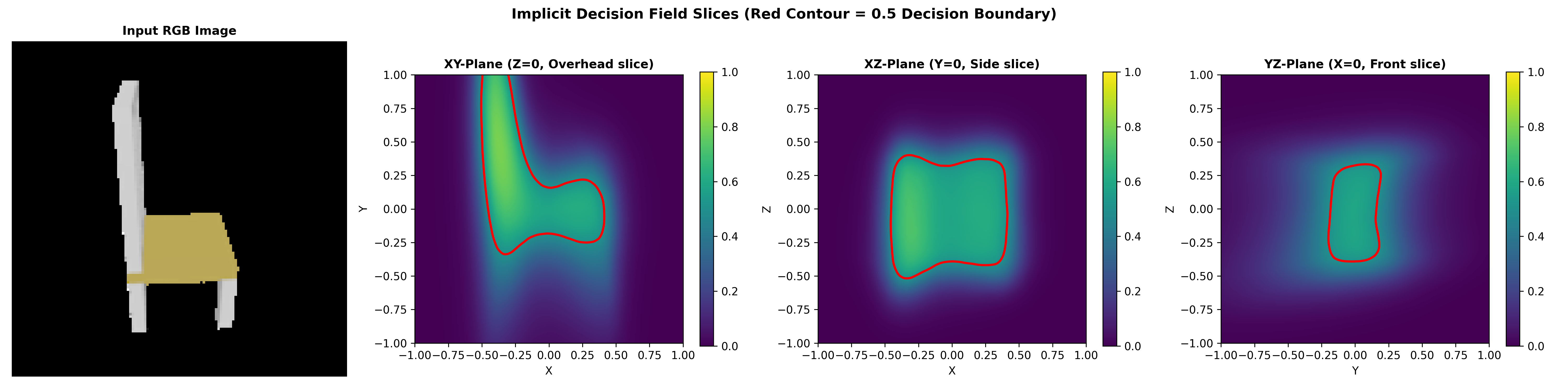
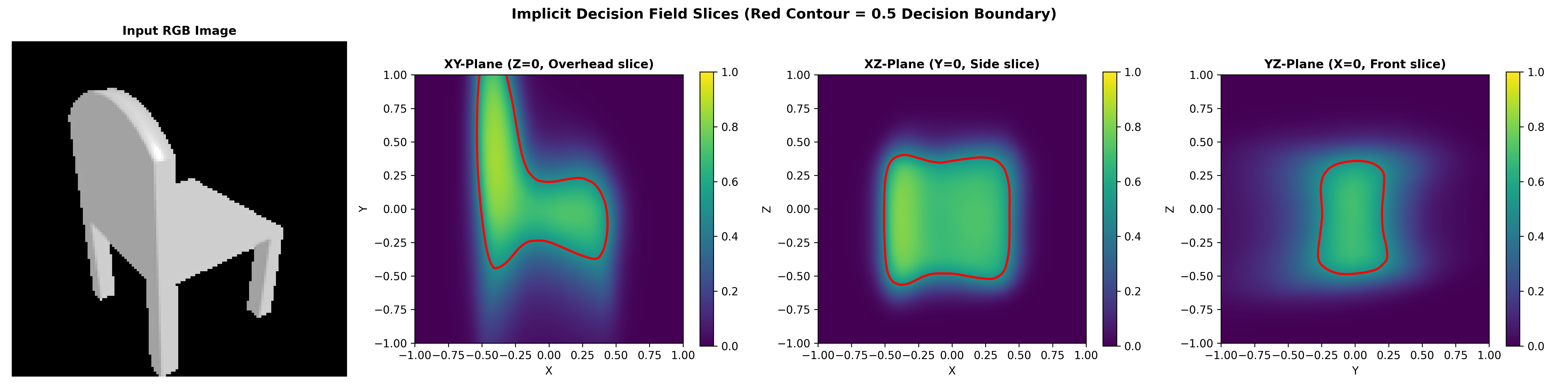
We can see how the seat and back of the chair are learned but the legs of the chair are not articulated enough and have a lower field value. This behaviour seems to be caused by the inherent smoothing and low-pass filtering of MLPs. Fourier positional encoding seems like it could be helpful here.
3. Exploring other architectures
3.1: Implicit network
| Input RGB | Ground truth | Predicted |
|---|---|---|
 |
 |
 |
 |
 |
 |
 |
 |
 |
Avg F1@0.05: 7.548
F1 score plot:
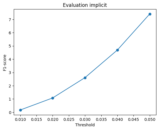
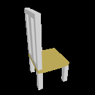
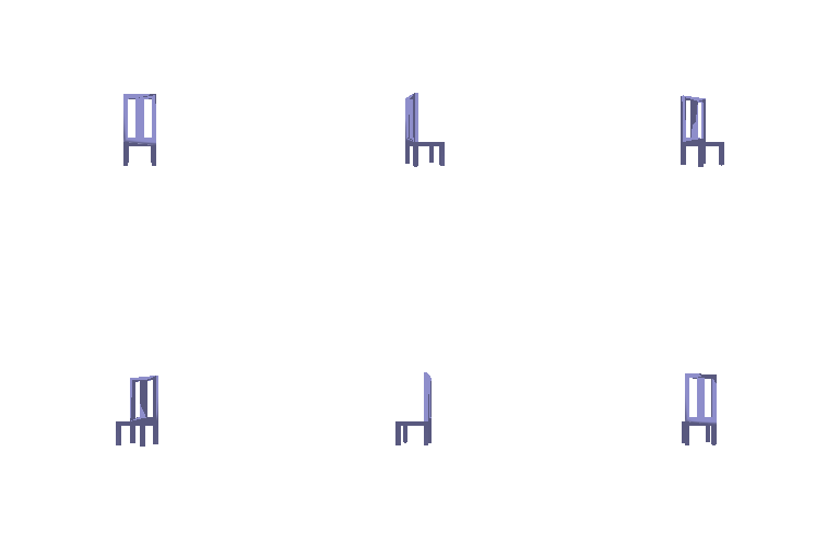
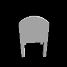
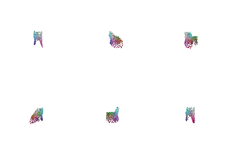
The outputs and visualizations show how the model learns a very smooth implicit field function and struggles to model the higher frequency details such as chair legs and slots in the backrest.
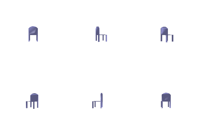
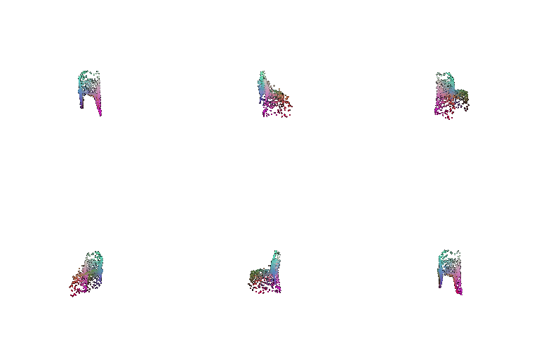
3.2: Parametric network
| Input RGB | Ground truth | Predicted |
|---|---|---|
 |
 |
 |
 |
 |
 |
 |
 |
 |
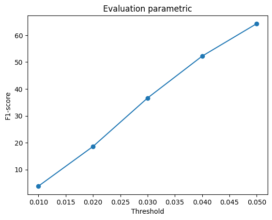
Avg F1@0.05: 64.318
F1 score plot:
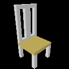
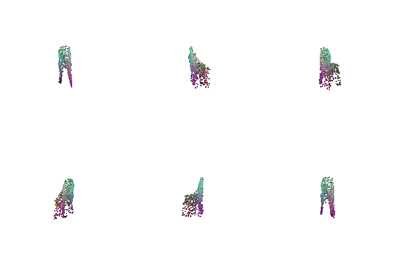
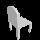
The outputs clearly show how the model tries to "drape" a 2D plane on the chair's 3D surface but fails at doing so at sharp geometry. (Maybe creating a more complex manifold to start off with can provide the model better opportunities to fit higher frequency surface details?)