1.1 Fitting a voxel grid
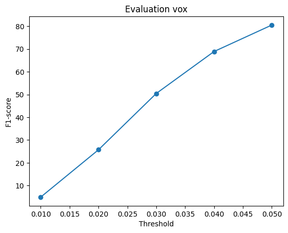
Binary cross entropy loss is used to predict the occupancy value of each voxel.


By Teja Kanthamneni · 16-825 Learning for 3D Vision
Fitting 3D representations and reconstructing chairs from one RGB image.
These experiments fit a 3D representation directly to a target. Each pair shows the optimized result and ground truth.
Binary cross entropy loss is used to predict the occupancy value of each voxel.
Symmetric Chamfer distance loss is used to match each predicted point to its nearest target point and each target point to its nearest prediction.
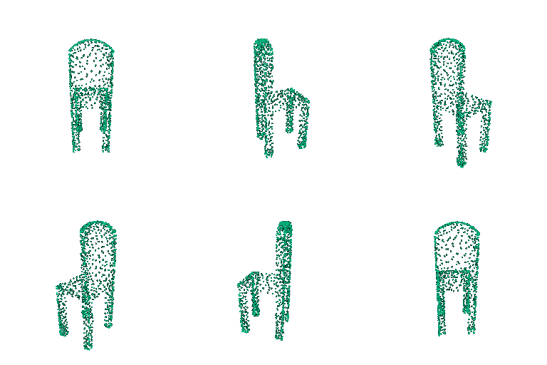

Combination of Chamfer distance and Laplacian smoothing make up the loss for the predicted mesh.


The voxel decoder consists of several nn.ConvTranspose3d layers. At a distance threshold of 0.05, the mean F1 score is 80.51%.


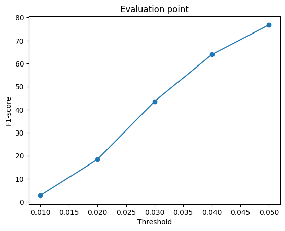
The point cloud decoder consists of several widening MLP layers to predict 10000 points. At 0.05, the mean F1 score is 76.81%.


The mesh decoder aslo uses several widening MLP layers to predict a deformation of a mesh. At 0.05, the mean F1 score is 71.38% for smoothness weight 0.1.


| Representation | F1 at 0.05 | What the representation can capture |
|---|---|---|
| Voxel grid | 80.51% | Occupancy and topology without a fixed mesh template; limited by grid resolution. |
| Point cloud | 76.81% | Flexible surface samples; no explicit faces or continuous surface. |
| Mesh (smoothness 0.1) | 71.38% | Connected surface; the starting topology and smoothness term restrict thin or separate parts. |
F1@0.05 counts an evaluation point as matched when its nearest point on the other shape is less than 0.05 away in 3D reference coordinates. In these runs, the voxel model likely scores highest because it predicts occupancy throughout a 3D grid without a fixed surface topology. The point cloud can place points freely on chair parts, but its finite samples leave gaps. The mesh starts from a connected sphere and is deformed into the target shape. The nature of this process makes it difficult to capture smooth surfaces, even with the smoothness loss term. Additionally the smoothness loss can also be working against the model by marking harder to capture edges, corners, and then components.
The mesh experiments vary the weight on the smoothness loss w_smooth. F1@0.05 decreases as the weight increases across these five runs. A stronger penalty can suppress narrow legs and other fine chair details that help surface overlap. While w_smooth = 0 performed the best, the surfaces, as expected, were quite jagged. There may be some middle ground between 0 and 0.1 for the smoothness weight, but given that with w_smooth = 0.1 the predicted mesh is still not very smooth, it is likely that wouldn't result in much improvement.
| Smoothness weight | Mean F1 at 0.05 |
|---|---|
| 0 | 74.24% |
| 0.1 | 71.38% |
| 0.5 | 69.75% |
| 1 | 68.15% |
| 5 | 61.50% |
Mean scores are from each run's saved evaluation CSV, using 1,000 sampled points.


Each caption reads colored shape → comparison target. For every visible vertex or point on the colored shape, we measure the 3D Euclidean distance to the nearest location on the target. A mesh target uses its triangle surfaces and a point-cloud target uses its nearest discrete point. A voxel-grid target is first converted to a triangle boundary surface; faces shared by two occupied voxels are removed. It is then treated like a mesh target. Mesh and voxel colors are computed at vertices and interpolated across faces, while point-cloud colors are assigned to individual points.
| Color | Distance to the comparison target |
|---|---|
| Green | 0: the colored geometry lies on the target. |
| Yellow | 0.05 units away. |
| Red | 0.10 units away or farther. |
Colors blend between those values and stop changing beyond 0.10. Intuitively, red on a prediction captures incorrect geometry in the prediction, while red on the ground truth captures geometry the prediction misses. All views use test sample 0, view 0.


Overall, this visualization technique is good at capturing areas of the ground truth mesh that the models struggled to capture and the excesses created by the model that don't exist in the ground truth. While this information could be determined without this gradient texture, highlighting the differences makes them significantly easier to determine.
This parametric point cloud model learns 25 different mappings that morph points from 2D planes into the object's 3D shape. We sample points on each of these planes during training and evaluation. This configuration allows us to sample different numbers of points at inference, unlike the original point cloud model, which is limited to the fixed number of points it was trained to predict. At 1,000 sampled points, its mean F1 at 0.05 is 75.76%, which is comparable to that of the original point cloud model. At 2,500, 5,000, and 10,000 sampled points, mean F1 at 0.05 increases to 76.86%, 78.83%, and 79.02%, respectively. However, this parametric model took about twice as long to train as the original.


