Setup
Environment Setup

Data
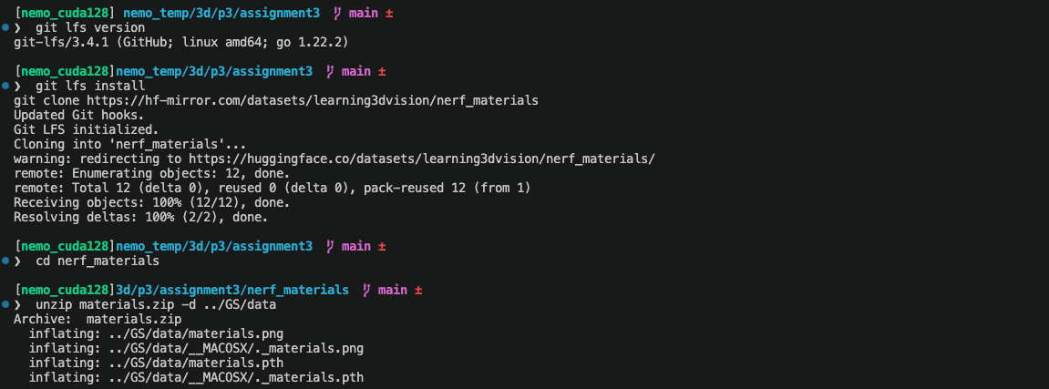

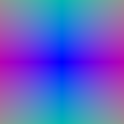
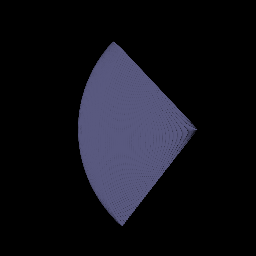

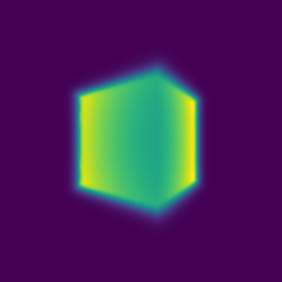






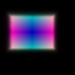

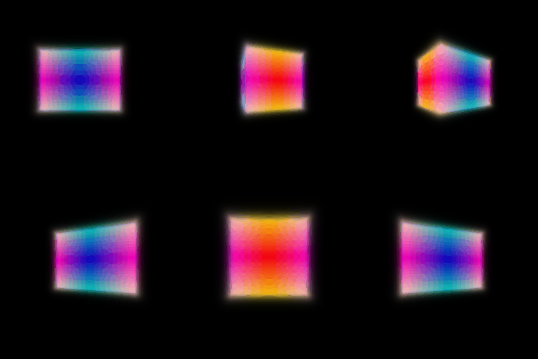
implicit.py and used mean squared error for RGB supervision in train_nerf.
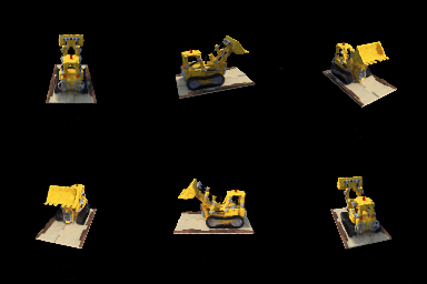
I extended NeRF to predict view-dependent color while keeping density dependent only on spatial position. The network takes a sampled 3D position (𝐱) and a normalized ray direction (𝐝), and outputs density (σ(𝐱)) and RGB color (𝐜(𝐱, 𝐝)).
The position is encoded using six harmonic frequencies and passed through eight fully connected hidden layers, each with 256 neurons and ReLU activation. A skip connection concatenates the position encoding with the input to the fifth hidden layer. The resulting features feed two branches: a linear density head followed by ReLU to ensure nonnegative density, and a linear feature head for color prediction.
The normalized direction is encoded using four harmonic frequencies and concatenated with the position features. A small color network, consisting of a 128-neuron ReLU hidden layer and a three-channel sigmoid output layer, predicts RGB values in [0, 1]. Direction information enters only this color branch, allowing appearance to vary with viewpoint without directly changing the predicted density.
For comparison, I used a position-only baseline with the same architecture and parameter count, replacing the direction embedding with zeros. This isolates the effect of direction conditioning. Both models use the same ray sampling and volume rendering pipeline and are trained with RGB mean squared error.
Implementation. Both models were trained on the materials dataset at 128×128 resolution for 300 epochs, using Adam with an initial learning rate of 10−4. Each iteration sampled 1,024 rays, with 128 points per ray between distances 1 and 7. The models used the same architecture, data splits, and random seed, differing only in whether direction information was provided to the color branch. We compared their validation MSE, PSNR, and rendered GIFs at epoch 300.


| Model | Validation MSE ↓ | Validation PSNR ↑ |
|---|---|---|
| Position-only Baseline | 0.004079 | 23.895 dB |
| View-dependent NeRF | 0.003197 | 24.953 dB |
Both models use their best-validation checkpoints (best.pt).

Discussion and Conclusion. Adding viewing direction improved performance on the materials scene. At epoch 300, the view-dependent model achieved a validation PSNR of 24.953 dB, compared with 23.895 dB for the baseline, and reduced validation MSE by approximately 21.6%. This indicates that direction conditioning benefited held-out viewpoints rather than only fitting the training images.
View dependence helps represent changing highlights and reflections, but an overly expressive direction branch may memorize training views and generalize poorly. Our design limits direction conditioning to a small color branch while keeping density dependent only on position.
Overall, the view-dependent model performed better under the tested settings. However, sharp highlights and complex reflections remained blurred, showing that direction conditioning alone does not fully recover detailed material appearance.
I implemented hierarchical sampling using two independently parameterized NeRF networks. The coarse network first evaluates 64 stratified samples along each ray. Its volume rendering weights define a probability distribution used to draw 64 additional samples through inverse-CDF sampling. The original and additional samples are merged and sorted, and the fine network evaluates all 128 points to produce the final color.
The sampling weights are detached when generating new sample locations. Both networks are trained using RGB supervision: MSE(Ccoarse, CGT) + MSE(Cfine, CGT).
I compared a single-network uniform sampling baseline with the coarse/fine model on the materials dataset. Both were trained at 128×128 resolution for 300 epochs, using Adam with an initial learning rate of 10−4 and 1,024 rays per iteration. Both used the same view-dependent network architecture per network, data splits, and random seed.
The baseline evaluated 128 samples per ray. The hierarchical model evaluated 64 coarse samples and 128 merged samples with the fine network, totaling 192 network evaluations per ray. Both methods used stratified perturbation during training and deterministic sampling during evaluation.
Experiments ran sequentially on the same otherwise-idle NVIDIA A100 40GB GPU. Rendering time was measured on the same validation camera after warm-up, using the median of five measurements.
| Method | Validation MSE ↓ | Validation PSNR ↑ | Training time ↓ | Rendering time per image ↓ |
|---|---|---|---|---|
| Uniform | 0.003253 | 24.878 dB | 61.32 min | 237.15 ms |
| Coarse/Fine | 0.003102 | 25.083 dB | 115.19 min | 340.46 ms |


Both models use their best-validation checkpoints (best.pt).
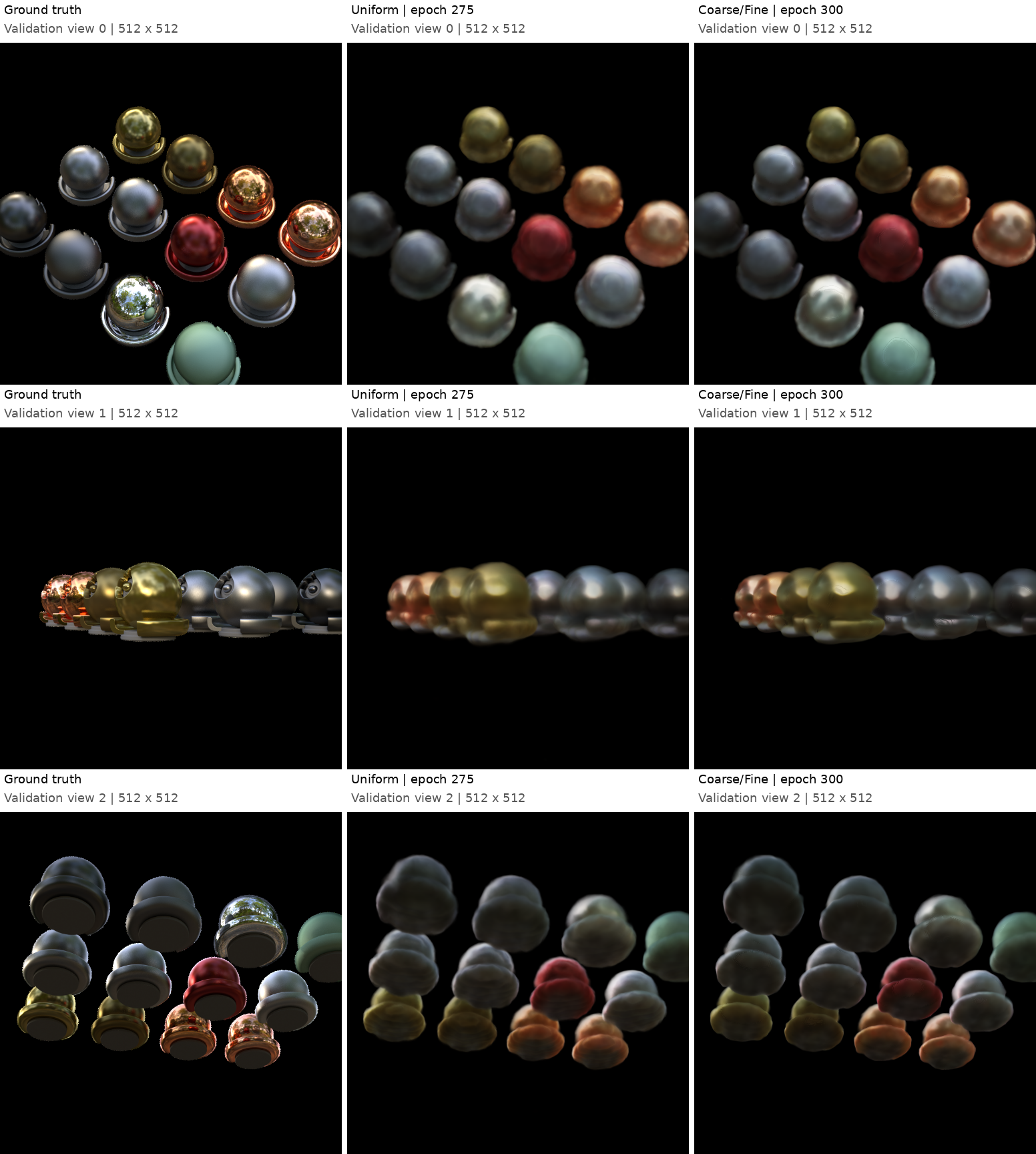
Hierarchical sampling concentrates additional samples in regions that contribute strongly to the rendered image. In this experiment, it provided a modest quality improvement, but training took approximately 1.88× as long and rendering time increased by 43.6%.
The hierarchical model uses both additional network evaluations and a second independently trained network, so the comparison measures the complete coarse/fine strategy rather than sampling alone. Under these settings, uniform sampling offered a better speed–quality trade-off, while coarse/fine sampling achieved slightly higher reconstruction quality at greater computational cost.
Implementation. I implemented separate MLPs for signed distance and color prediction using positional encoding. The distance network has six linear layers with hidden width 128, while the color network has two linear layers with hidden width 128. The SDF output is unconstrained, allowing negative values inside the object and positive values outside. The color output uses a sigmoid activation. For the distance network, I used Softplus hidden activations and geometric initialization to start from an approximately spherical SDF, initially suppressing the weights associated with the harmonic input features.
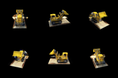
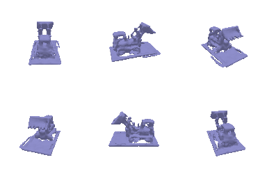
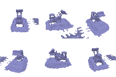
Experimental settings. I trained on the Lego bulldozer dataset at 128×128 resolution for 250 epochs per experiment. I compared β ∈ {0.01, 0.02, 0.05, 0.10, 0.20}, keeping α = 10, the Eikonal weight at 0.02, and the network architecture fixed. Each training iteration sampled 1,024 rays, with 128 points per ray between distances 2 and 6. The initial learning rate was 5×10⁻⁴.


Selected result. I selected β = 0.01 as the best overall setting based on the rendered colors and extracted geometry. It produced a relatively clean appearance while retaining a more complete base and recognizable bulldozer structure. The reconstruction is not perfect: small holes and rough surface details remain. These conclusions are based on qualitative inspection of the rotating renderings.
Interpretation of α and β. The parameter α sets the density scale: increasing it increases light attenuation inside the object. The parameter β controls the width of the density transition around the surface. Larger values create a broader transition, while smaller values make the transition sharper.




 β=0.02
β=0.05
β=0.10
β=0.20
A larger β allows appreciable density farther outside the zero level set. Consequently, the model can explain image appearance using a wider transition region, and the learned surface may shift or lose geometric detail. A smaller β ties the density boundary more closely to the SDF zero level set. This does not imply that changing β always causes a particular direction of expansion or contraction.
A moderately larger β generally provides useful density gradients over a wider spatial region, which can make optimization easier. With a small β, the transition is narrow and requires sufficiently dense sampling near the surface. Our uniform sample spacing is approximately 4/127 ≈ 0.0315, so the β=0.01 experiment is particularly sensitive to sampling. However, the final renderings alone do not establish which setting converged faster.
With adequate sampling and successful optimization, a smaller β can support more precise surface localization because the density transition is sharper. In these experiments, β=0.01 gave the best qualitative balance, whereas β=0.20 produced substantial geometric artifacts. The results were not strictly monotonic: β=0.10 had cleaner color renderings than β=0.05, but its geometry still contained visible holes. This also shows why both color and geometry should be evaluated.
Already completed in model.py.
Already completed in model.py.
 All test cases have passed.
Already completed in model.py.
Already completed in model.py.
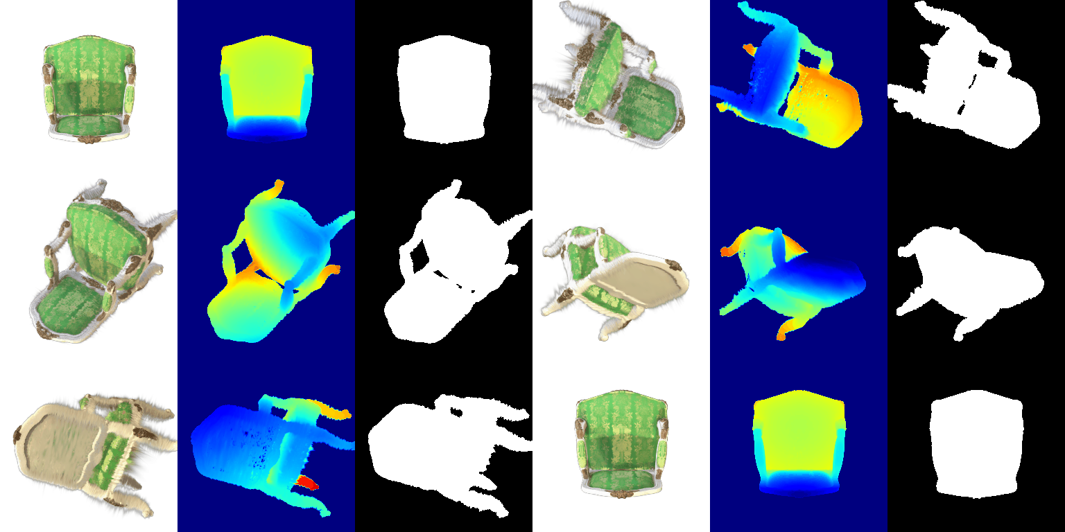
Already completed in train.py.
I trained the isotropic Gaussian representation of the toy truck for 4,000 iterations, using the Adam optimizer and an L1 loss between the rendered images and the ground-truth images.
The learning rates were:
| Parameter | Learning rate |
|---|---|
| Means | 0.00016 |
| Scales | 0.003 |
| Colours | 0.0025 |
| Opacities | 0.025 |
Evaluation on the held-out test views produced a mean PSNR of 31.031 dBand a mean SSIM of 0.951. This configuration achieved higher scores than my initial 1,000-iteration experiment, which obtained 29.146 dB PSNR and 0.937 SSIM Both the learning rates and the iteration count changed between the experiments.
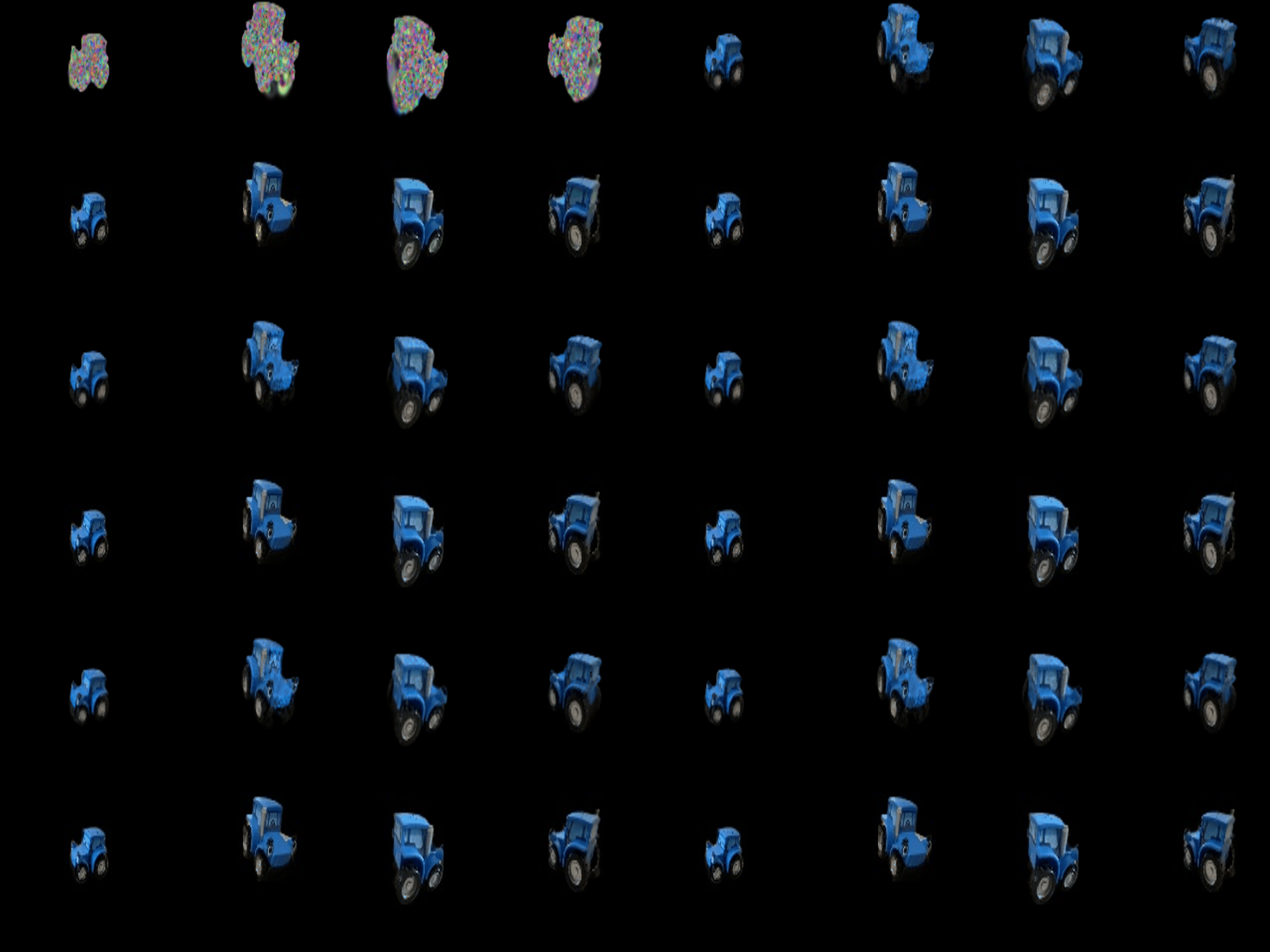
The following GIFs show the training progress and the final rendered views. In the training progress GIF, the top row shows the predicted renderings, while the bottom row shows the ground-truth images.



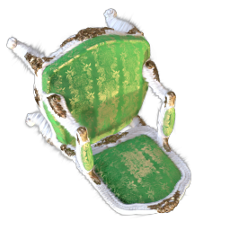


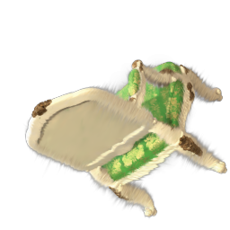

For column 1, the rendering with spherical harmonics (7.1) shows darker green upholstery, especially on the seat, than the DC-only rendering (5.5). The chair’s overall shape remains unchanged.
For column 2, the backrest and seat appear darker in 7.1, making the gold patterns stand out more against the green fabric. The DC-only rendering appears brighter and more uniform.
For column 3, the two renderings look very similar from the underside. Only subtle differences in shading are visible around the seat base and frame.
For column 4, the front-facing backrest is noticeably darker in 7.1, increasing the contrast between the green fabric and the gold patterns. The silhouette remains consistent between the two renderings.
| ID | Gaussian Type | Loss Function | Iterations | Learning Rate Schedule | PSNR ↑ | SSIM ↑ |
|---|---|---|---|---|---|---|
| A | Isotropic | L1 | 1,000 | Fixed | 17.585 | 0.645 |
| B: Official Baseline | Isotropic | L1 | 4,000 | Fixed | 18.517 | 0.687 |
| C | Isotropic | L1 | 10,000 | Decay to 10% of the initial value | 18.504 | 0.686 |
| D: Highest PSNR | Isotropic | L1 | 10,000 | Fixed | 18.680 | 0.704 |
| E | Isotropic | L1 + SSIM | 6,000 | Fixed | 18.355 | 0.704 |
| F | Anisotropic | L1 + SSIM | 6,000 | Fixed | 18.497 | 0.709 |
| G: Highest SSIM | Anisotropic | L1 + SSIM | 10,000 | Fixed | 18.575 | 0.715 |
| Setting | Baseline | Final Method |
|---|---|---|
| Initialization | Random, 10,000 Gaussians | Random, 10,000 Gaussians |
| Gaussian Type | Isotropic | Anisotropic |
| Loss Function | L1 | 0.8 × L1 + 0.2 × (1 − SSIM) |
| Optimizer | Adam | Adam |
| Position / Scale Learning Rate | 0.00016 / 0.003 | 0.00016 / 0.003 |
| Color / Opacity Learning Rate | 0.0025 / 0.025 | 0.0025 / 0.025 |
| Rotation Learning Rate | N/A (rotation not optimized) | 0.001 |
| Training Iterations | 4,000 | 10,000 |
| Learning Rate Decay | None | None |
| Mean PSNR (dB) | 18.517 | 18.575 |
| Mean SSIM | 0.687 | 0.715 |
The model represents the materials scene using 10,000 randomly initialized anisotropic 3D Gaussians. Each Gaussian has a learnable position, three independent scale parameters, a rotation quaternion, an RGB color, and an opacity. The independent scales and rotation allow each Gaussian to vary its shape and orientation.
For each camera view, the renderer filters out Gaussians with negative depth, sorts the remaining Gaussians from front to back, and projects them onto the image plane. It computes per-pixel alpha values and transmittance, then blends the Gaussian colors to produce the predicted image.
The model is trained with the combined objective: L = 0.8 × L1(Ipred, Igt) + 0.2 × (1 − SSIM(Ipred, Igt)). Both terms are differentiable, allowing gradients to propagate through the renderer to the Gaussian parameters. Training uses Adam for 10,000 iterations with fixed learning rates: 0.00016 for positions, 0.003 for scales, 0.0025 for colors, 0.025 for opacities, and 0.001 for rotations. Scales use an exponential activation, opacities use a sigmoid activation, and rotation quaternions are normalized before rendering. The number of Gaussians remains fixed throughout training, with no adaptive densification or pruning.
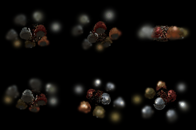
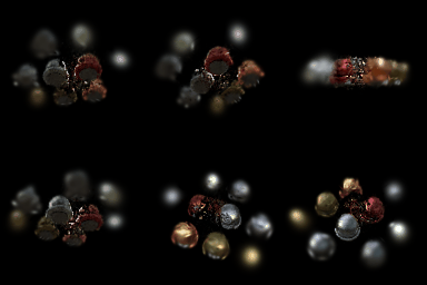
Compared with the baseline using the Q6.2 training setup, my final method increases training from 4,000 to 10,000 iterations, replaces isotropic Gaussians with anisotropic Gaussians, and uses a combined loss of 0.8 × L1 + 0.2 × (1 − SSIM). The anisotropic representation also optimizes quaternion rotations with a learning rate of 0.001. Both methods use random initialization with 10,000 Gaussians and fixed learning rates.
The final method improves PSNR from 18.517 to 18.575 dB and SSIM from 0.687 to 0.715. I selected this method because it achieves the highest SSIM among my experiments. However, the isotropic L1 method trained for 10,000 iterations achieves the highest PSNR, at 18.680 dB, so no single configuration performs best on both metrics.
The experiments show that longer training improves the fixed-learning-rate L1 results. At 6,000 iterations with the same combined loss, anisotropic Gaussians improve both PSNR and SSIM over isotropic Gaussians. In contrast, decaying all learning rates to 10% of their initial values does not improve the results in this experiment.
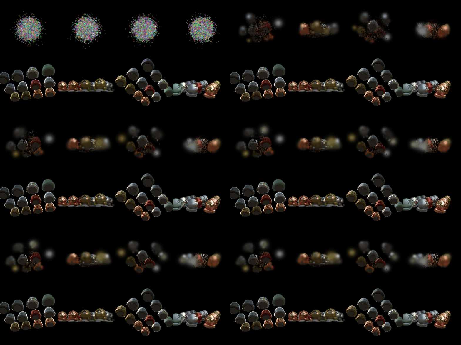
The GIFs show the progression from random initialization to a recognizable reconstruction. Both methods still exhibit blurred objects and visible artifacts, so the improvement remains limited. Since the final method changes the training duration, loss function, and Gaussian type together, its improvement over the baseline cannot be attributed to any one modification alone.