2. Reconstructing 3D from single view (80 points)
2.1. Image to voxel grid (20 points)
The model checkpoint for this task is cps/checkpoint_vox.pth.
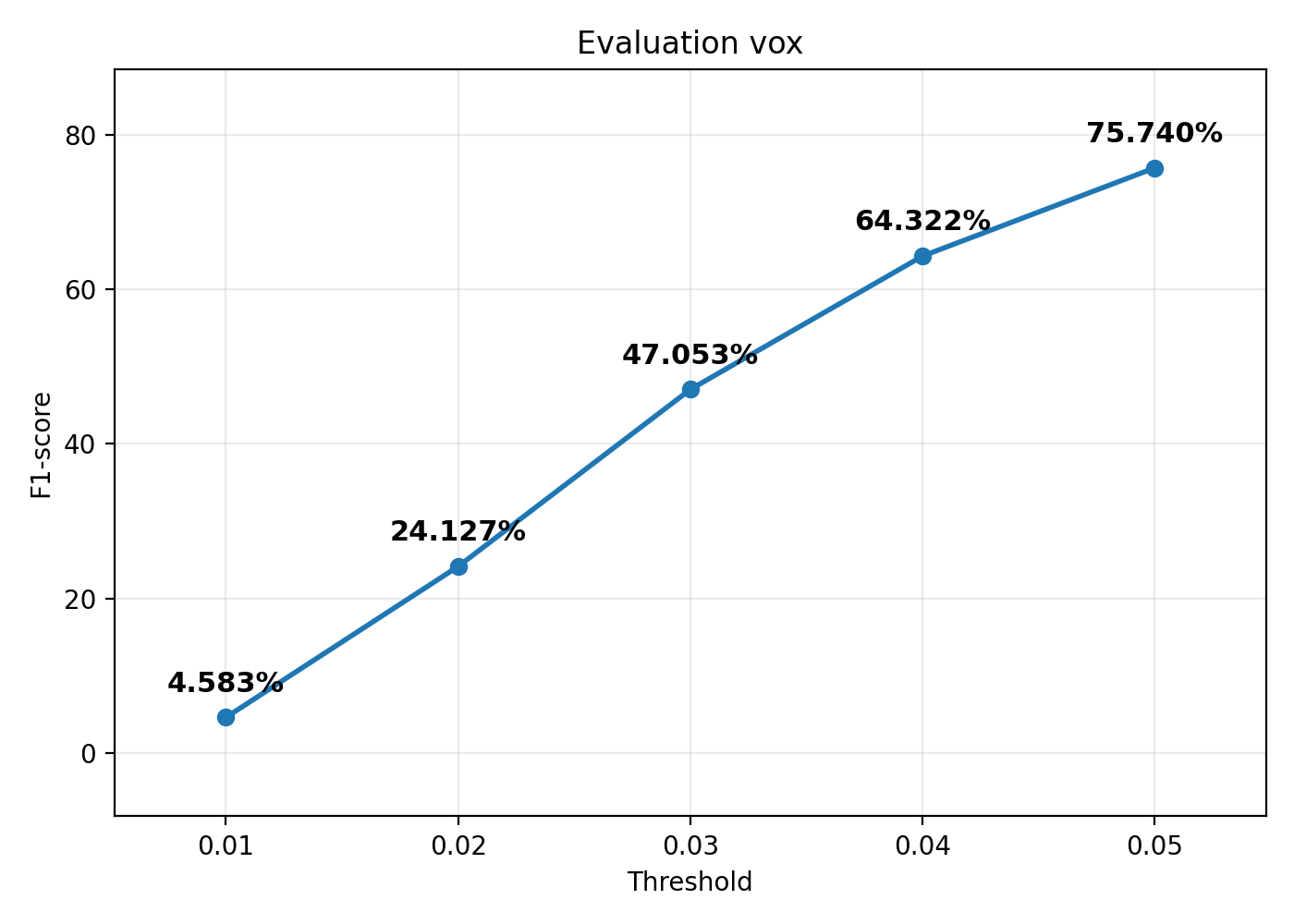
My model achieves an average F1@0.05 score of 75.740% on the test set. The plot above shows the average F1 scores at different distance thresholds.
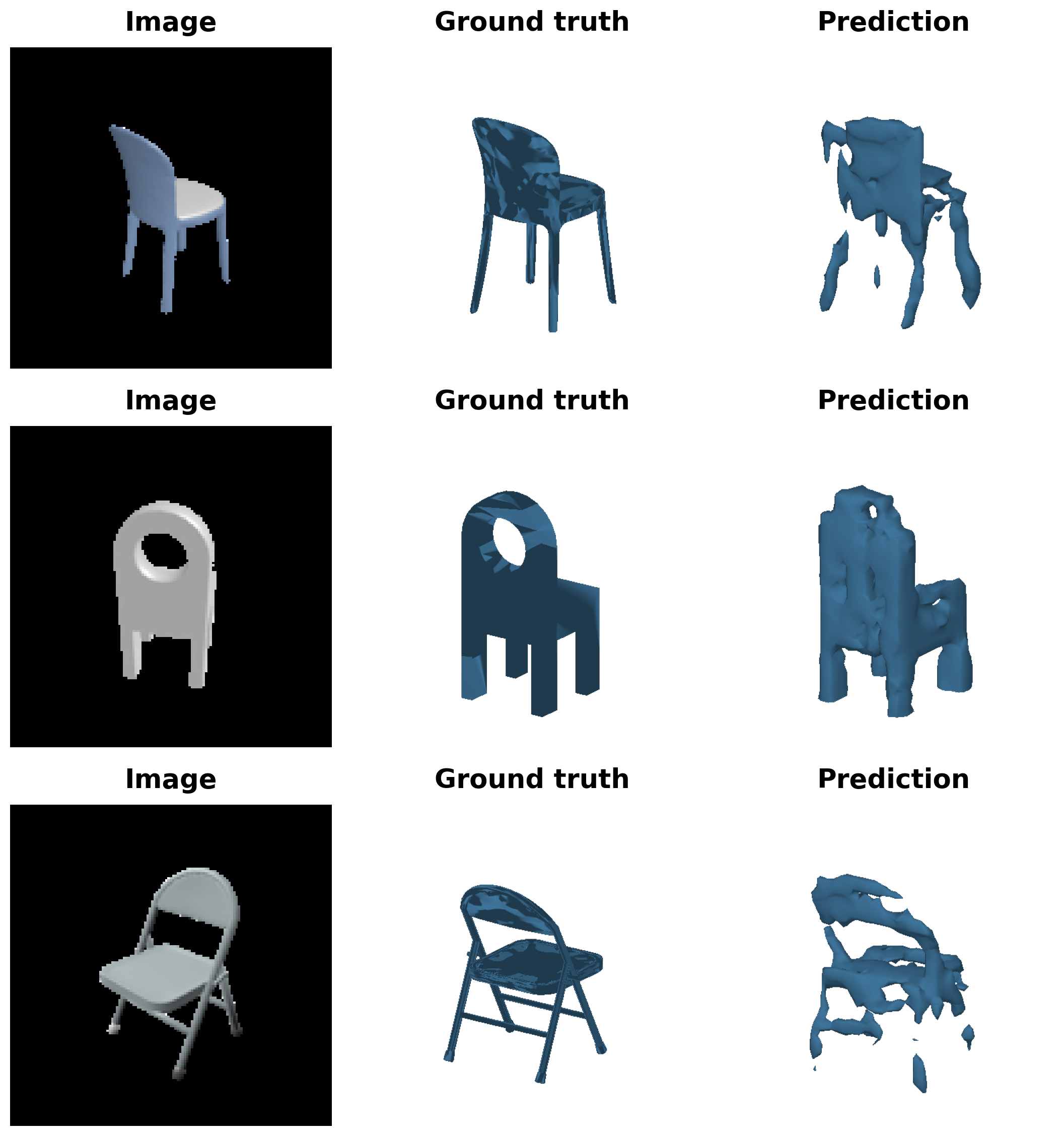
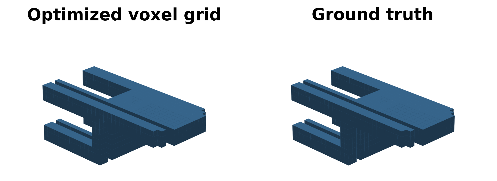
Qualitative results on three test examples. From left to right: input RGB image, ground-truth mesh, and the surface extracted from the predicted voxel grid using marching cubes. The predictions capture the overall chair shapes but exhibit missing thin structures, disconnected parts, and distorted details.
2.2. Image to point cloud (20 points)
The model checkpoint for this task is cps/checkpoint_point_1000.pth.
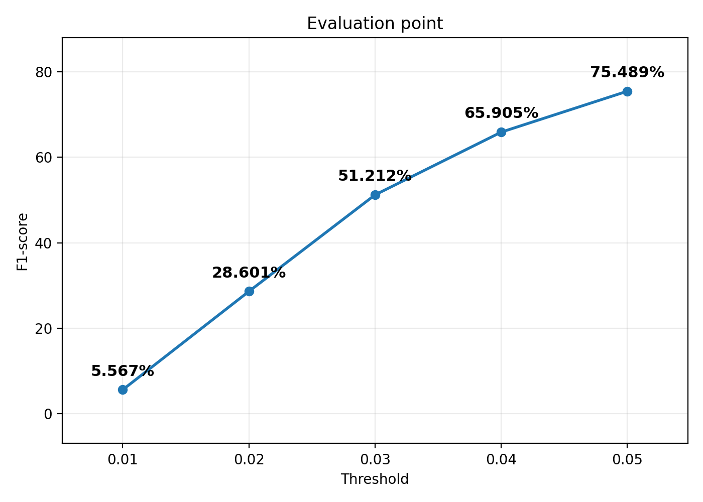
My point cloud model achieves an average F1@0.05 score of 75.489% on the test set. The plot above shows the average F1 scores at different distance thresholds.
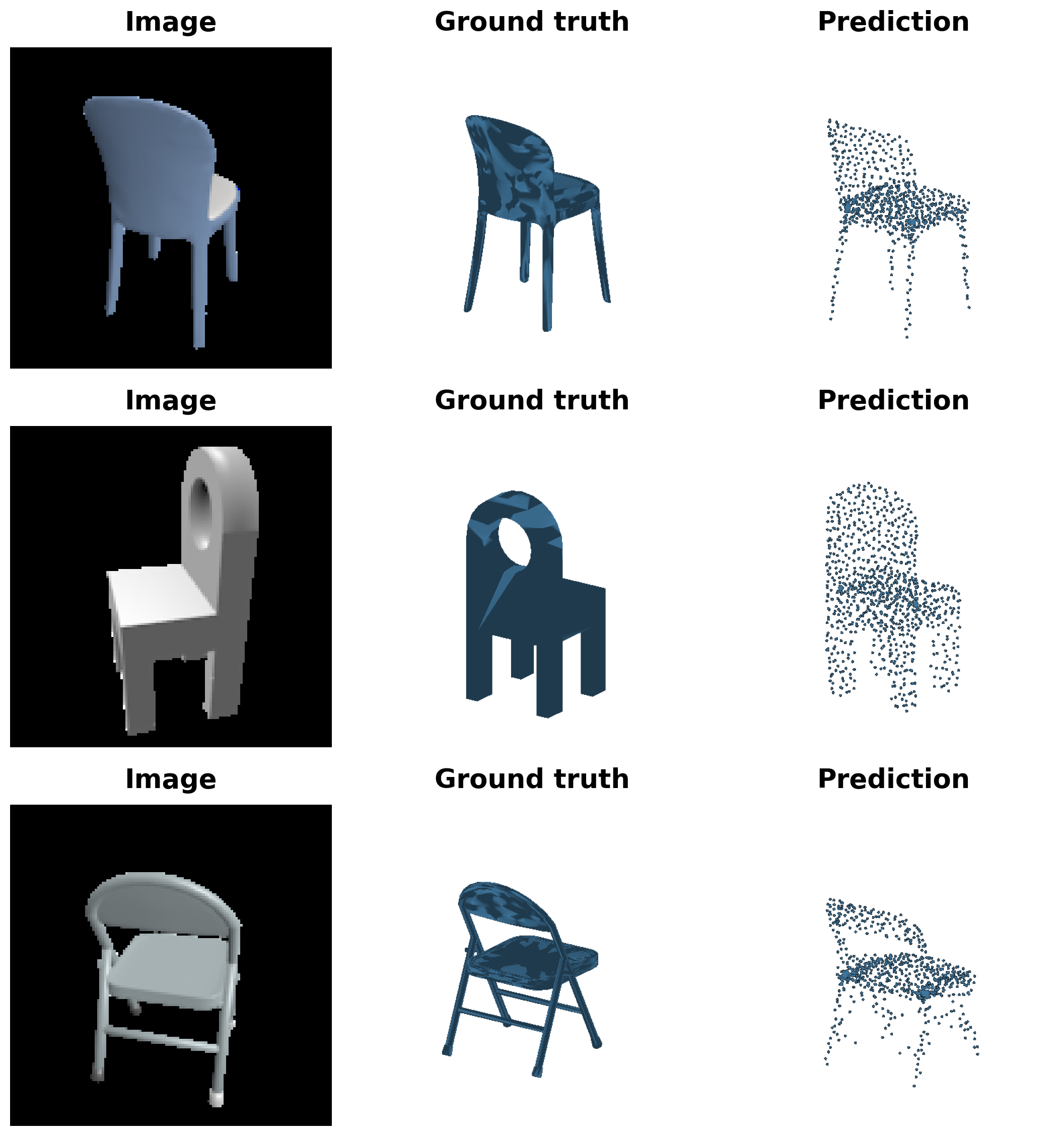
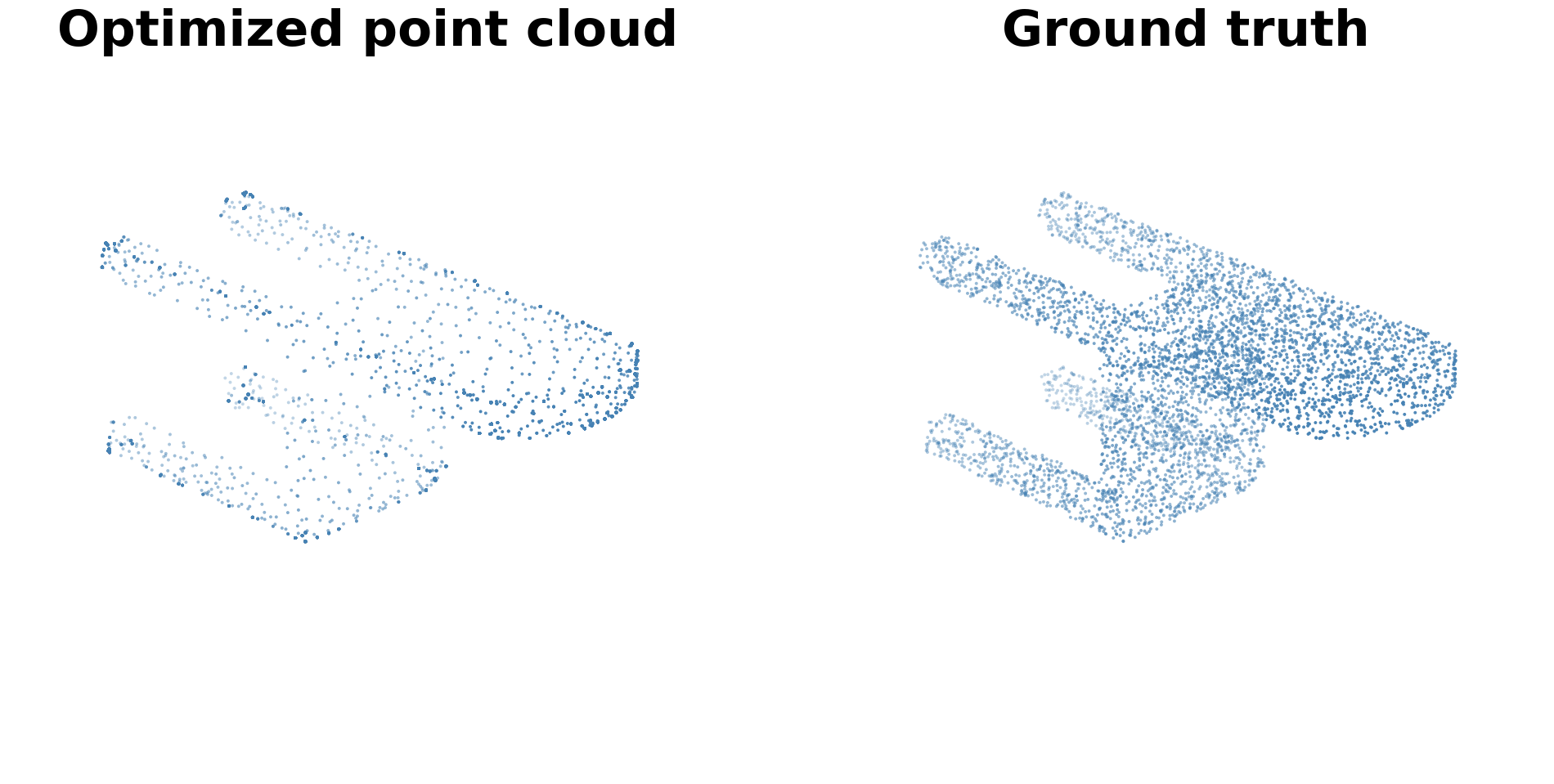
Qualitative results on three test examples. From left to right: the input RGB image, the ground-truth mesh, and the predicted point cloud. The predictions capture the overall chair shapes, including the backrests, seats, and legs. However, point coverage is uneven, thin structures are sparsely represented, and some details, such as the hole in the second chair’s backrest, are not clearly recovered.
2.3. Image to mesh (20 points)
The model checkpoint for this task is cps/checkpoint_mesh.pth.
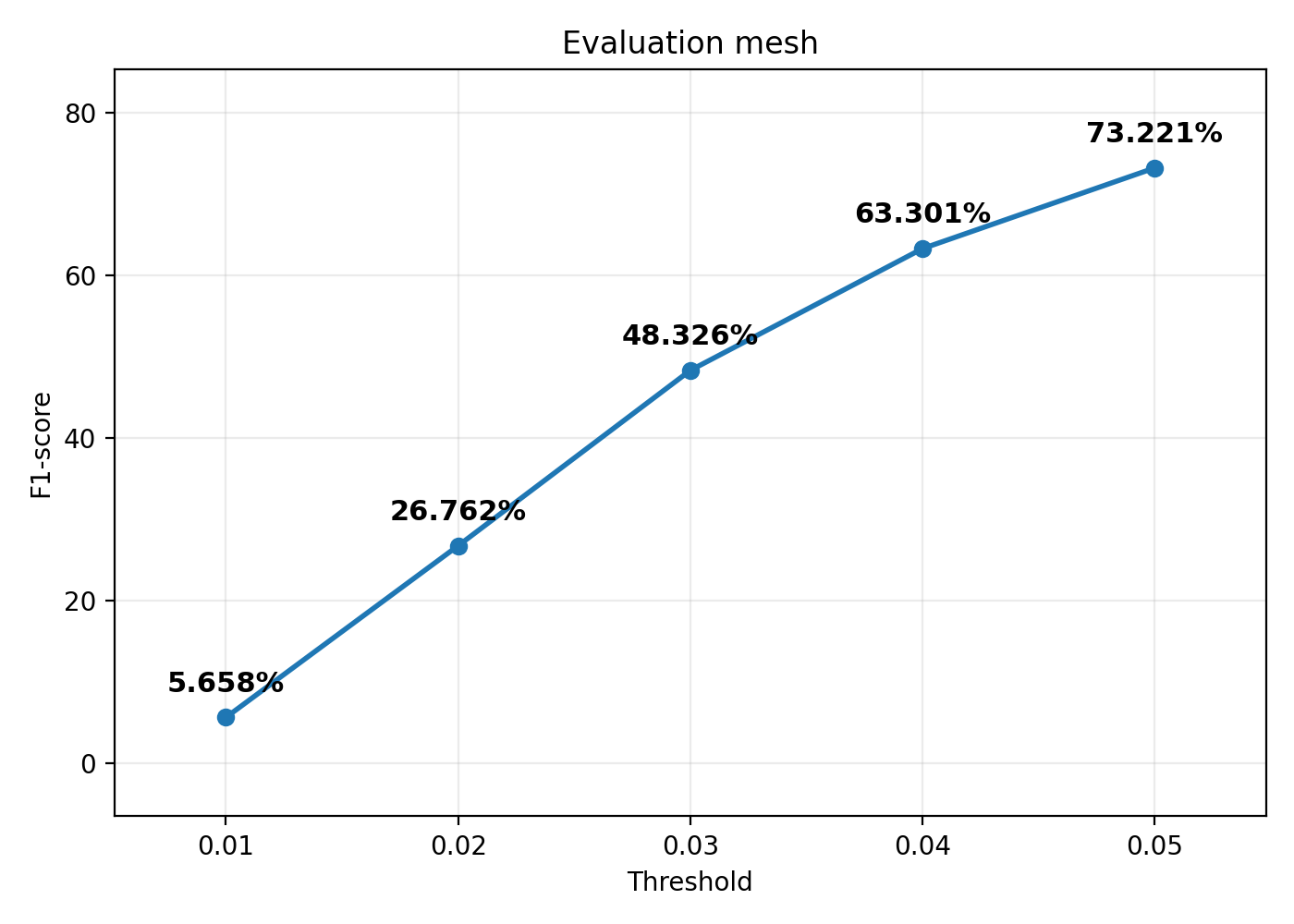
My mesh model achieves an average F1@0.05 score of 73.221% on the test set. The plot above shows the average F1 scores at different distance thresholds.
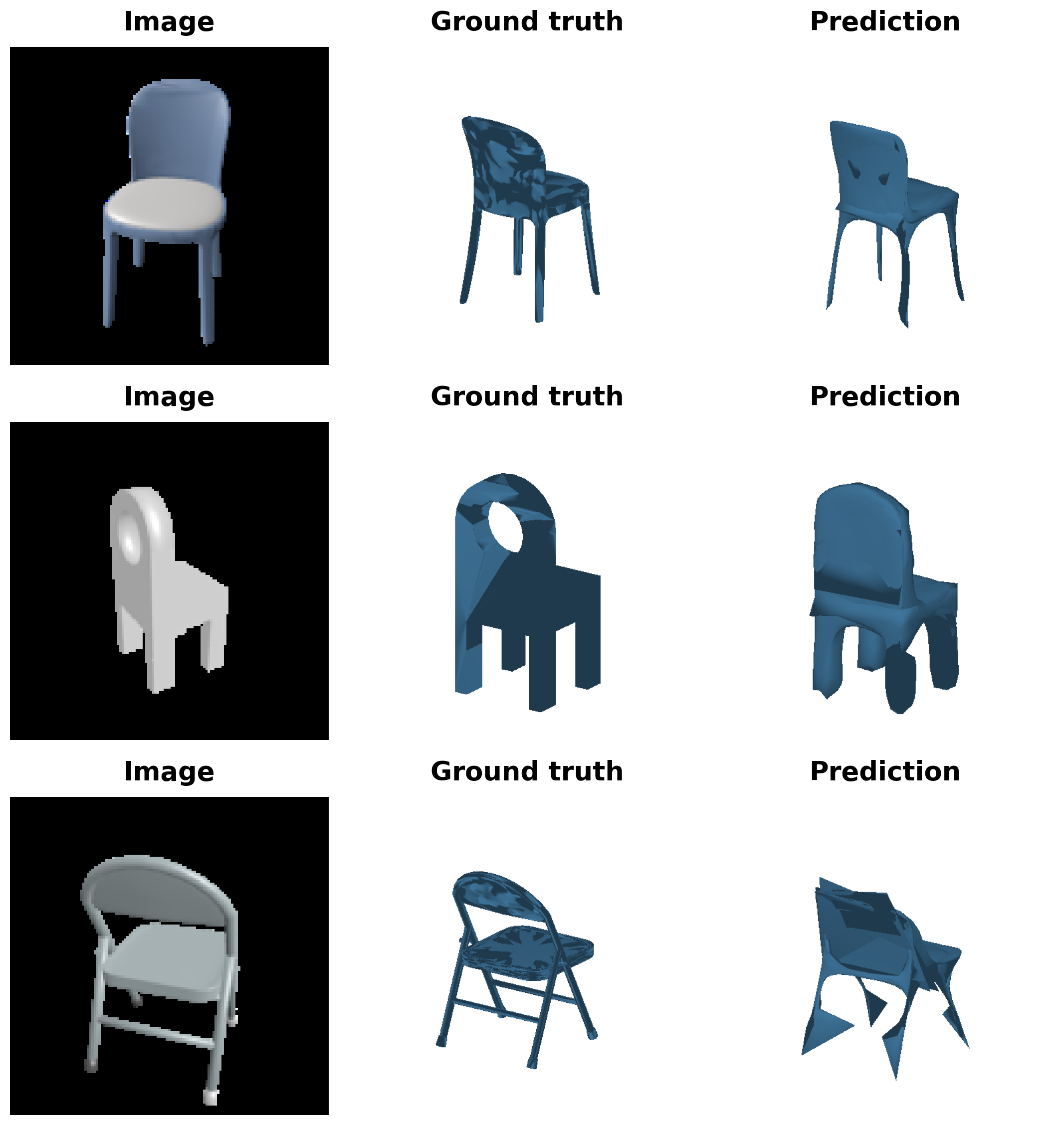
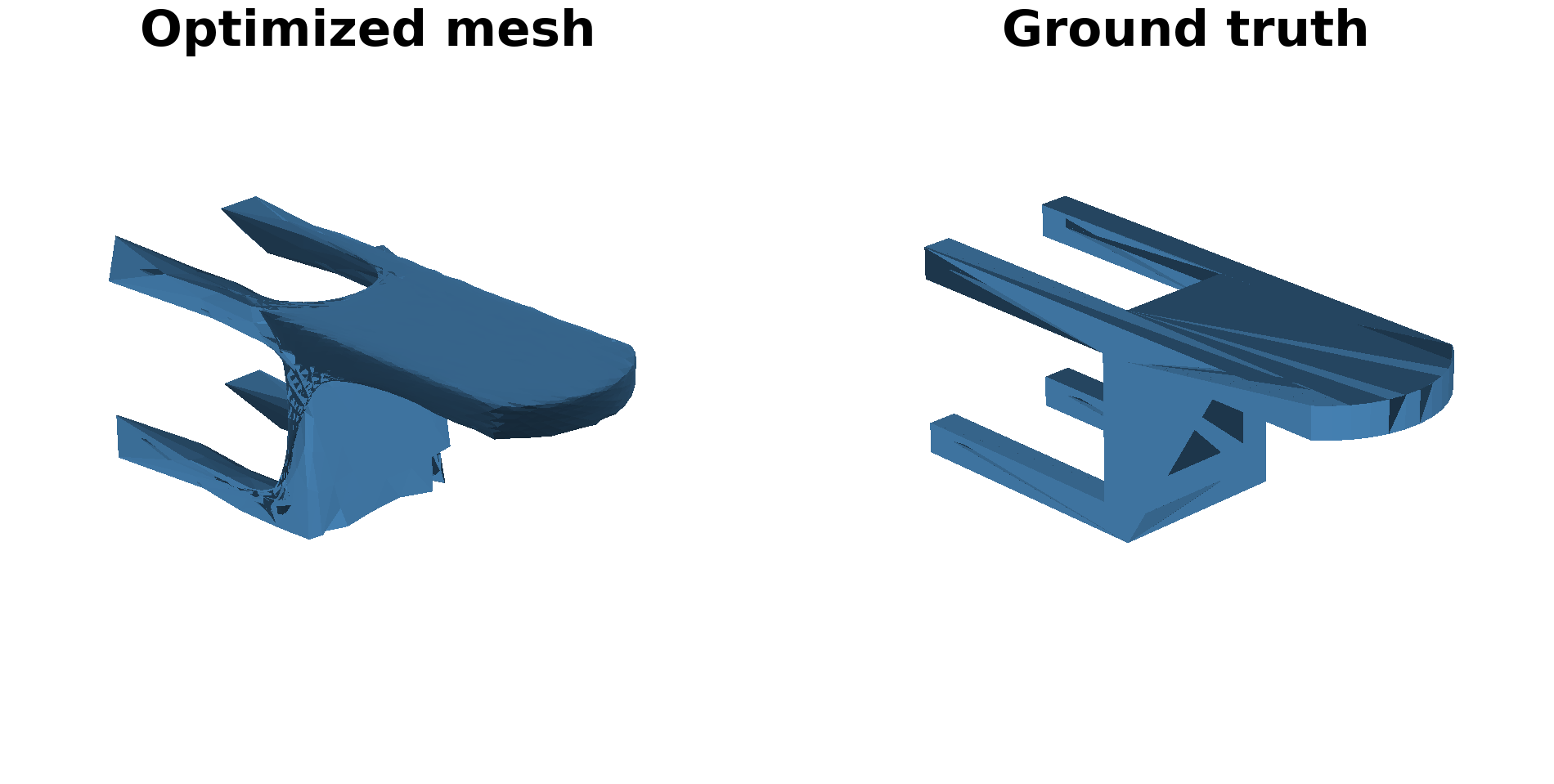
Qualitative results on three test examples. From left to right: the input RGB image, the ground-truth mesh, and the predicted mesh obtained by deforming an icosphere template. The predictions recover the overall chair shapes but struggle with fine geometric details. The hole in the second chair’s backrest is not recovered, while the third example exhibits stretched triangular faces and substantial distortions in the legs and backrest.
Comparison of 3D Representations
| Representation |
Mean F1@0.05 |
| Voxel grid |
75.740% |
| Point cloud |
75.489% |
| Mesh |
73.221% |
In the reported evaluations, the voxel model achieves the highest F1@0.05, but its advantage over the point-cloud model is only 0.251 percentage points. The mesh model scores 2.519 percentage points below the voxel model. However, the ranking depends on the distance threshold: the point-cloud model achieves higher F1 scores than both other models at thresholds of 0.02, 0.03, and 0.04. Therefore, these results do not indicate that one representation is consistently superior.
The visualizations highlight different limitations of the three approaches. The 32³ voxel grid provides a regular spatial representation, but its limited resolution makes thin structures difficult to preserve; the predictions contain missing or fragmented chair legs and supports. The point-cloud decoder places points directly in continuous 3D space, allowing flexible surface coverage, but the predicted points are unevenly distributed and some thin structures remain sparse. The mesh decoder produces connected surfaces by deforming an icosphere with fixed connectivity, but this restricts topology changes and can lead to stretched faces when fitting complex chair structures. These properties provide plausible explanations for the observed errors, although the experiments do not isolate their individual effects.
Overall, voxel and point-cloud reconstruction have similar reported F1@0.05 scores, while mesh reconstruction performs slightly worse in this experiment. These comparisons describe the trained models and evaluation runs shown here, rather than a universal ranking of the representations.
2.4. Analyse effects of hyperparams variations (10 points)
The model checkpoint for this task is cps/checkpoint_point_500.pth, cps/checkpoint_point_1000.pth, cps/checkpoint_point_2000.pth, cps/checkpoint_point_4000.pth, cps/checkpoint_point_6000.pth.
I investigate the effect of the number of predicted points on single-view 3D reconstruction by comparing models with 500, 1,000, 2,000, 4,000, and 6,000 output points. All experiments use the same encoder, decoder hidden layers, learning rate, batch size, number of training iterations, and training/test splits. The decoder’s output dimension and the number of ground-truth points sampled during training vary with the point count.
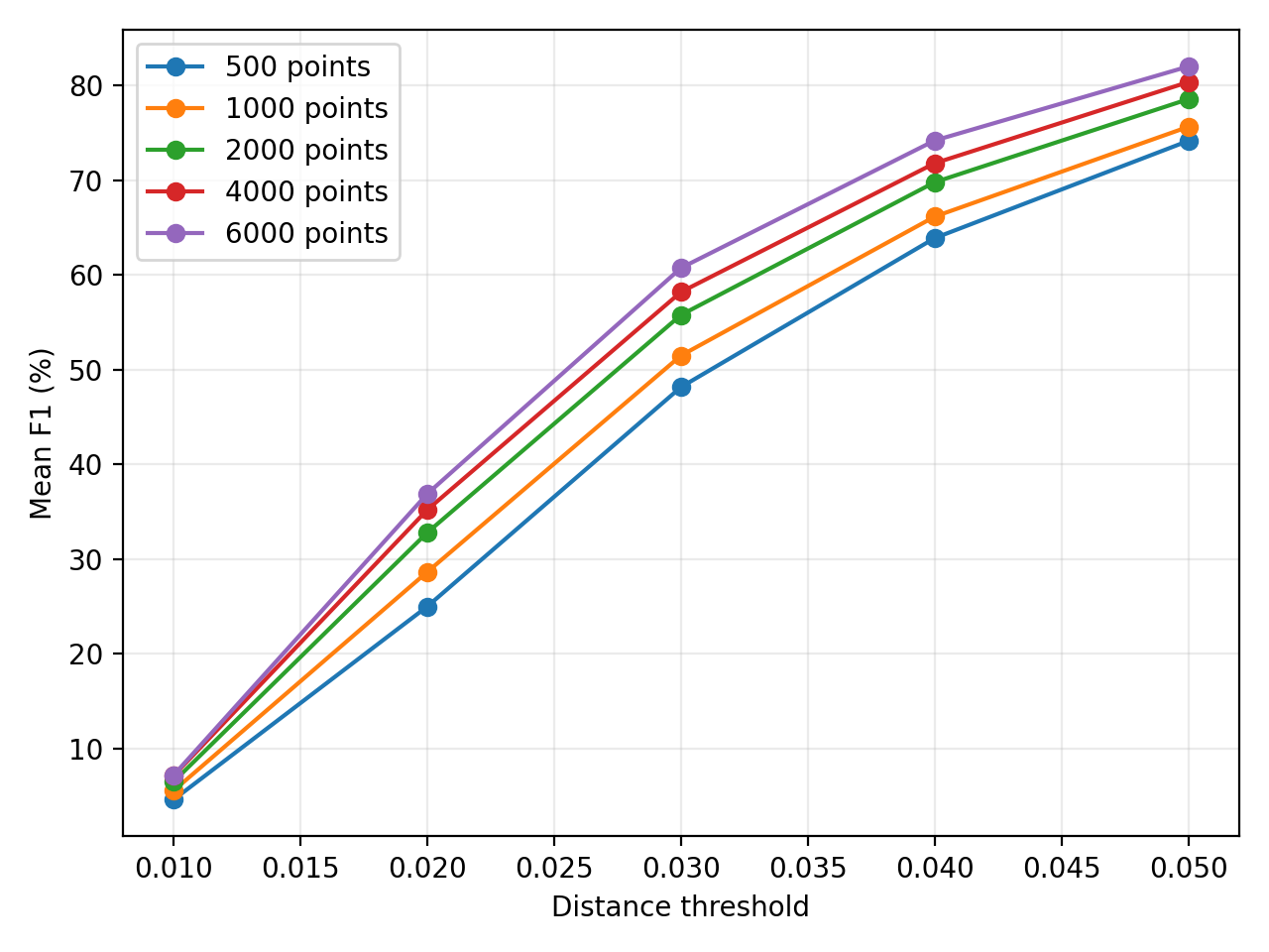
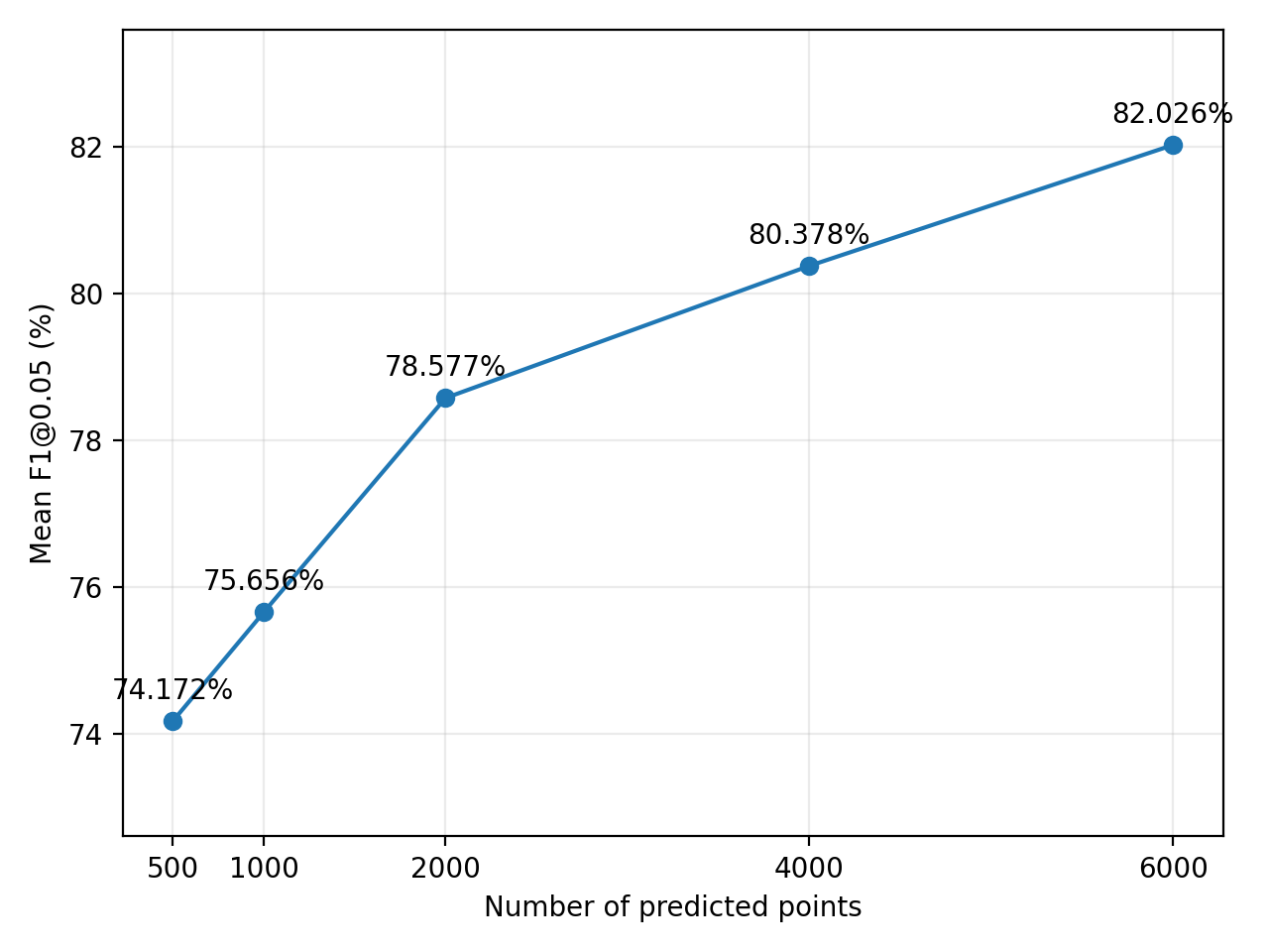
Increasing the number of predicted points improves the mean F1 score across all evaluated distance thresholds. F1@0.05 rises from 74.172% with 500 points to 82.026% with 6,000 points, an improvement of 7.854 percentage points. The gains become smaller per additional point at higher point counts: increasing from 2,000 to 4,000 points adds 1.801 percentage points, while increasing from 4,000 to 6,000 adds 1.648. Among the tested configurations, 6,000 points achieves the highest F1@0.05. However, denser predictions can improve nearest-neighbor coverage even without recovering finer geometric details, so these scores should be interpreted together with the visualizations.
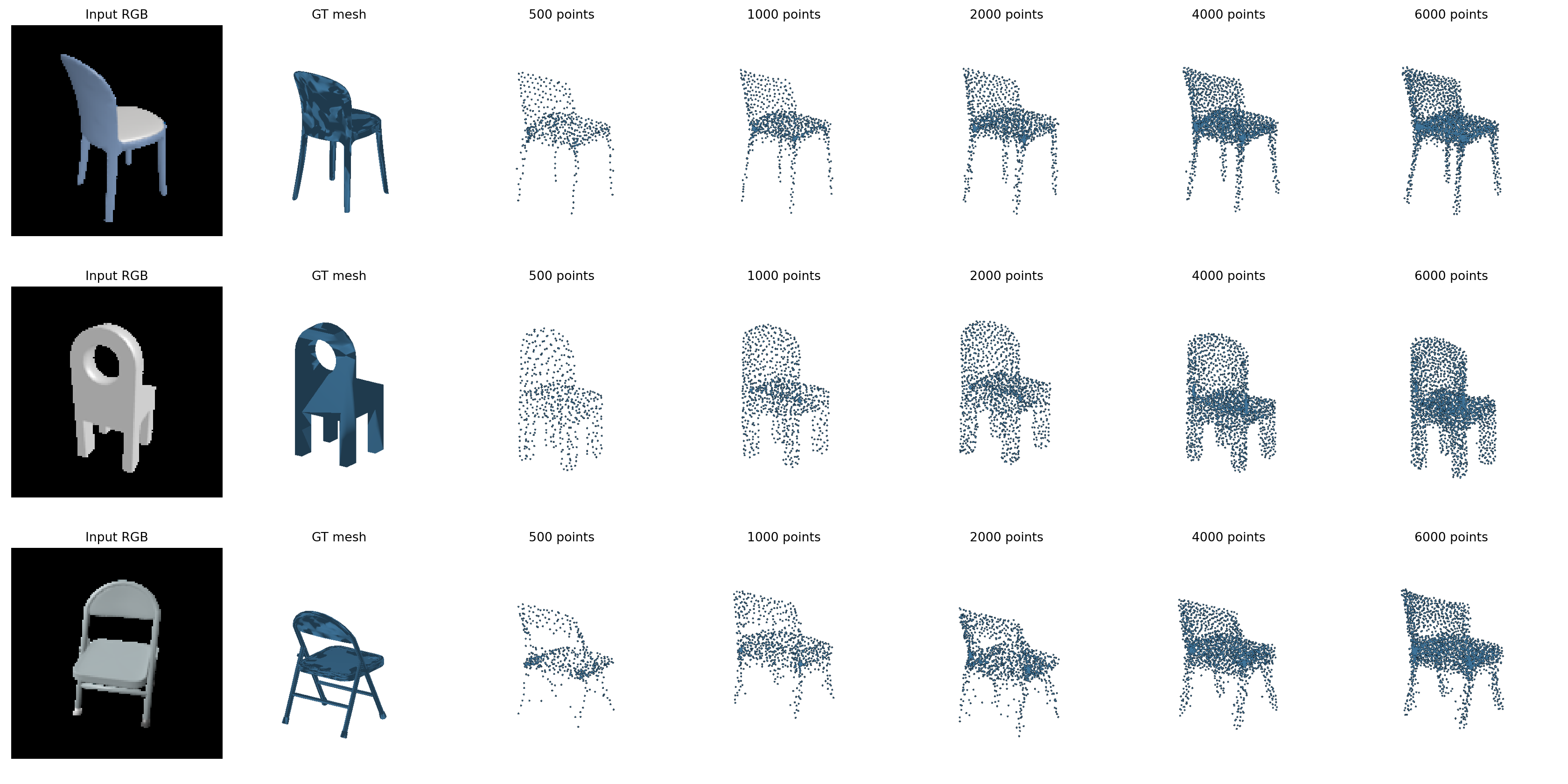
The qualitative comparison shows that larger point counts produce denser coverage of the predicted chair shapes, particularly around the seats and backrests. With 500 points, thin structures such as chair legs are sparsely represented; higher point counts make these structures easier to distinguish. However, increasing density does not consistently recover the correct geometry. The hole in the second chair’s backrest remains poorly reproduced, and the folding chair’s open frame and thin supports are not accurately recovered even with 6,000 points. Thus, increasing the point count improves coverage and the F1 score, but does not by itself resolve structural reconstruction errors.
2.5. Interpret your model (10 points)
The model checkpoint for this task is cps/checkpoint_point_1000.pth.
Model Design - Occlusion Sensitivity Experiment
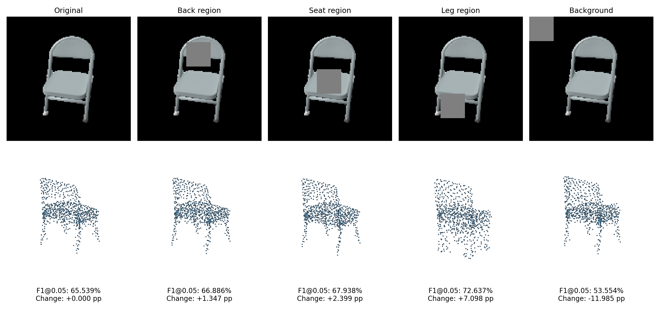
To investigate how the model responds to changes in its input, I perform an occlusion sensitivity experiment using the trained 1,000-point reconstruction model. For each of three test examples, I compare the original image with four variants containing an equally sized gray mask over an upper object region, a middle object region, a lower object region, or the background. The model weights, input viewpoint, and ground-truth point samples remain fixed across conditions. Predictions are rendered with the same camera and scale within each example. The reported change is the difference in F1@0.05 from the original input, measured in percentage points.
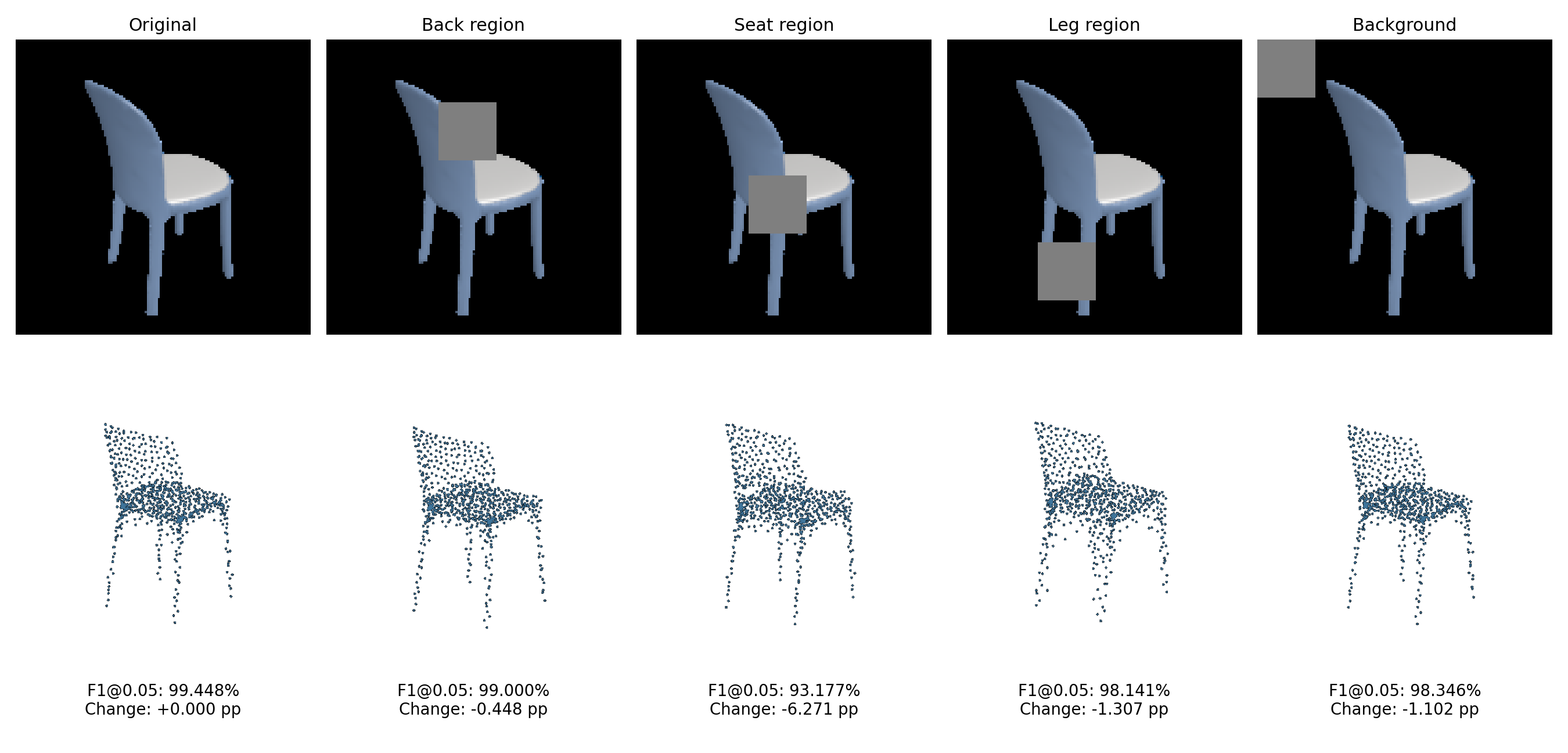
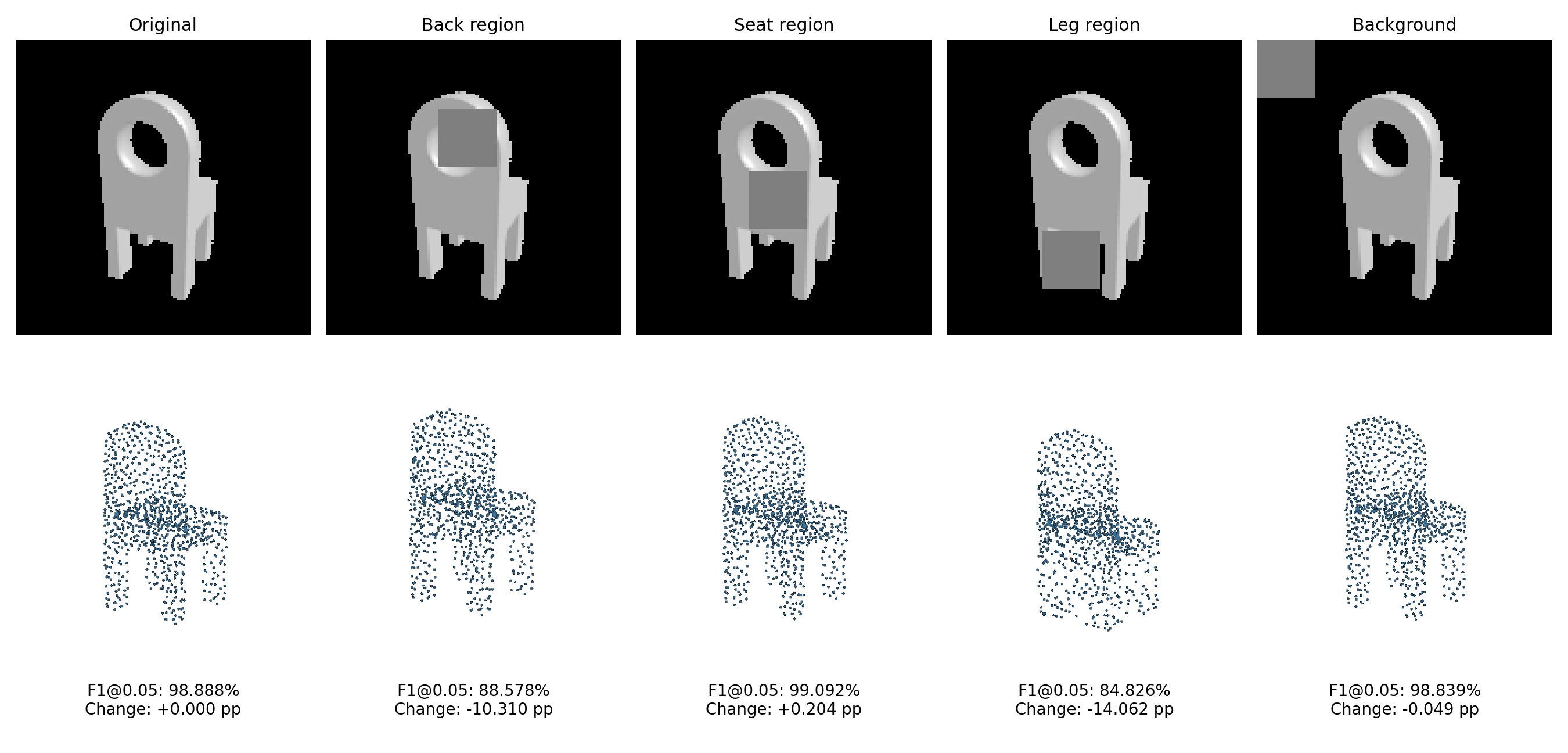
The effects of occlusion vary across examples and image regions. For the first chair, masking the middle region produces the largest F1 decrease, from 99.448% to 93.177% (−6.271 percentage points), while the other masks have smaller effects. For the second chair, masking the upper and lower regions reduces F1 by 10.310 and 14.062 percentage points, respectively. These results indicate that the model’s reconstruction depends on different visual cues for different inputs.
The folding chair shows a different pattern: masking the lower region increases F1 from 65.539% to 72.637%, whereas masking the background decreases it to 53.554%. Thus, removing image information does not always reduce this metric, and a background perturbation can substantially affect the predicted geometry. The higher F1 under lower-region occlusion does not establish that the reconstructed structure is better in every respect; the predicted supporting frame remains inaccurate.
Overall, the experiment reveals sensitivity to both object regions and background appearance. These observations apply to the three selected examples and the specific masks used. They do not establish a universal ranking of part importance or provide a direct visualization of the model’s attention.
3. Exploring other architectures / datasets. (Choose at least one! More than one is extra credit)
3.1 Implicit network (10 points)
The model checkpoint for this task is cps/checkpoint_vox_implicit_v2.pth.
Model Design
I implement an image-conditioned implicit occupancy network for single-view 3D reconstruction. A pretrained ResNet18 encoder extracts a 512-dimensional feature vector from the input RGB image. Given this feature and a 3D query coordinate, the decoder predicts a scalar occupancy logit.
The decoder augments each coordinate with sine and cosine features at four frequencies: π, 2π, 4π, and 8π. Together with the original coordinates, these form a 27-dimensional input, which is projected to 256 dimensions and added to a projected image feature. The resulting representation passes through four residual blocks of width 256. Each block incorporates a separate projection of the image feature and uses two linear layers with ReLU activations. A final ReLU and linear layer produce the occupancy logit. Decoder weights are shared across query locations.
I construct a 32 x 32 x 32 grid of voxel-center coordinates within (-1, 1)³. During training, 4,096 grid locations are uniformly sampled per iteration and paired with their corresponding ground-truth voxel labels. The encoder and decoder are trained jointly using binary cross-entropy with logits and a positive-class weight of 3 to increase the penalty for missing occupied locations. Training uses Adam with a learning rate of 0.0002, a batch size of 8, and 100,000 iterations. The gradient norm is clipped to 1.0.
During inference, all 32,768 grid locations are evaluated in chunks of 4,096. The logits are converted to occupancy probabilities using sigmoid and reshaped into a 32³ volume. Marching cubes extracts the surface at an occupancy threshold of 0.5 for visualization and geometric evaluation.
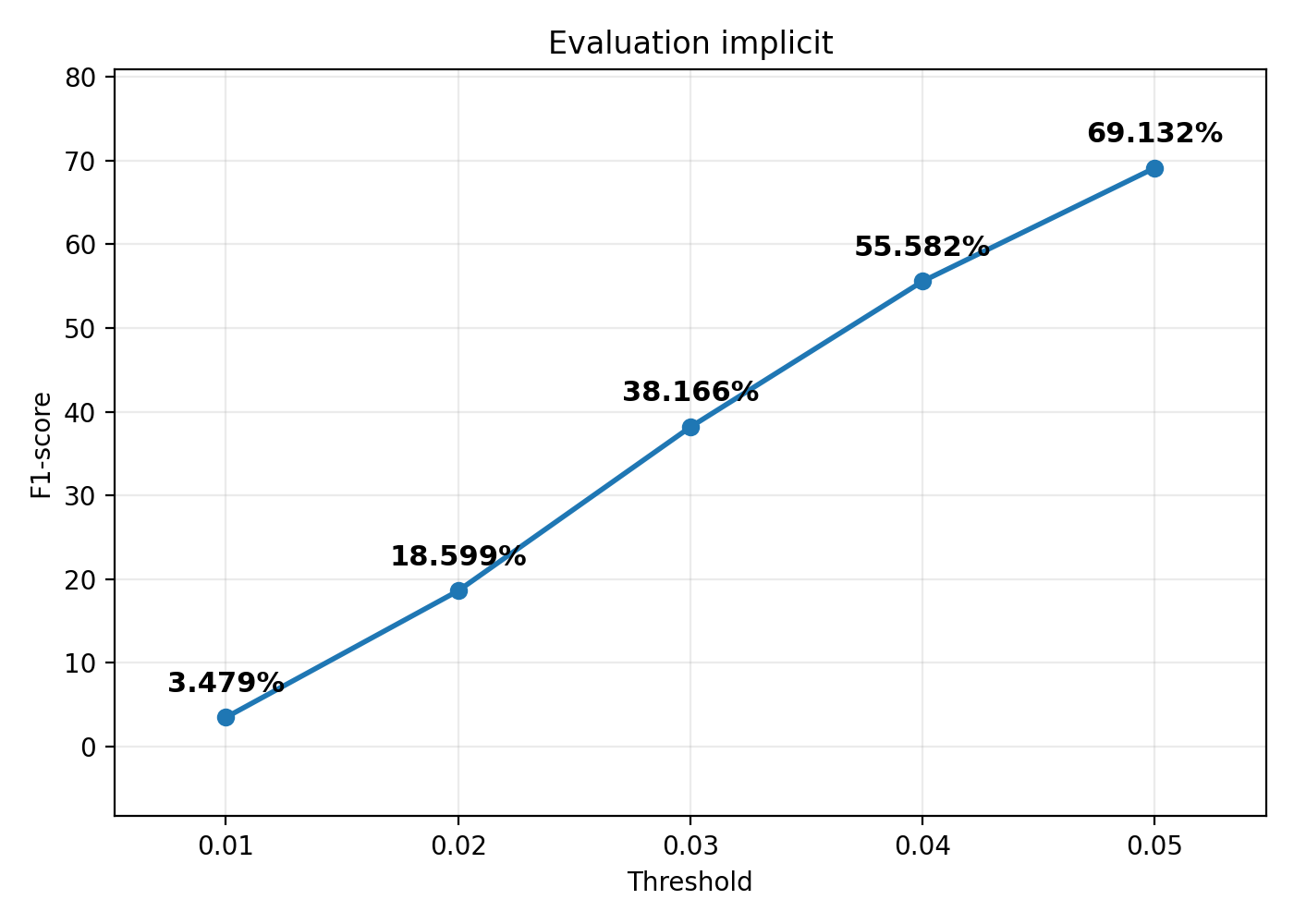
The implicit model achieves an average F1@0.05 score of 69.132% on the test set. The curve reports average F1 scores at different distance thresholds, increasing from 3.479% at 0.01 to 69.132% at 0.05. The much lower scores at stricter thresholds indicate that accurate surface localization remains challenging, even when the overall reconstructed shape is recognizable.
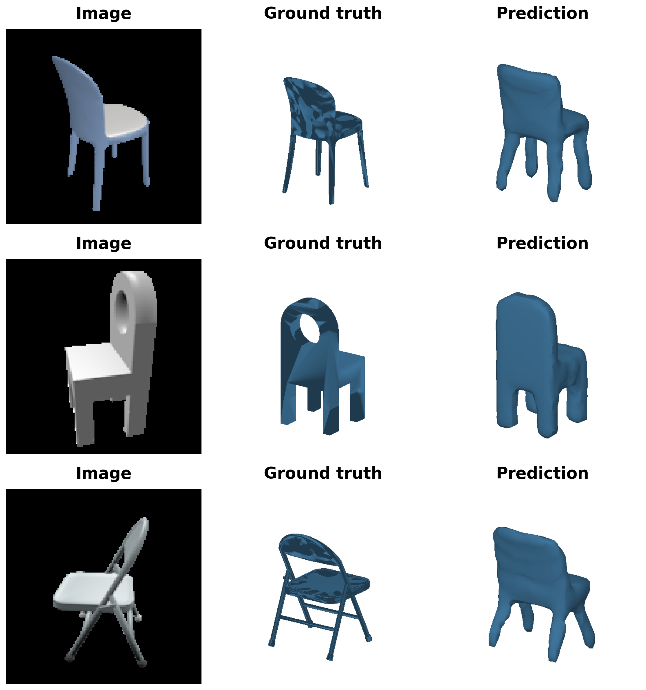
Qualitative results on three test examples. From left to right: the input RGB image, the ground-truth mesh, and the surface extracted from the predicted implicit occupancy field using marching cubes. The predictions capture the overall chair structure but have overly thick legs and simplified geometry. The hole in the second chair's backrest is missing, while the folding chair is reconstructed with a solid backrest and lacks its thin supporting bars.
These examples illustrate the distinction between producing a complete-looking shape and accurately recovering its surface geometry. Positive-class weighting may contribute to the more filled-in predictions by penalizing missed occupancy more strongly, but its individual effect has not been isolated experimentally.
3.2 Parametric network (10 points)
The model checkpoint for this task is cps/checkpoint_point_parametric_1000_p4.pth.
Model Design
I implement a simplified AtlasNet-style parametric network for single-view 3D reconstruction. A pretrained ResNet18 encoder extracts a 512-dimensional feature vector from the input RGB image. The decoder consists of four independently parameterized surface patches. Each patch maps a 2D coordinate (u, v), conditioned on the image feature, to a 3D point (x, y, z).
Within each patch, the image feature and the 2D coordinate are linearly projected to 256 dimensions and added together. This is equivalent to applying a linear layer to their concatenation. The resulting feature passes through an MLP with hidden widths of 256, 256, and 128, using ReLU activations, followed by a linear layer that outputs three coordinates. Network weights are shared across all query points within a patch, while different patches have separate weights.
During training, 250 coordinates are sampled uniformly from [-1, 1]² for each patch, producing 1,000 3D points in total. The encoder and decoder are trained jointly using a bidirectional squared-distance Chamfer loss between the predicted points and points sampled from the ground-truth mesh. During evaluation, fixed 2D samples are used to make the decoder output deterministic for a given image feature.
Unlike the baseline point decoder, which directly outputs a fixed list of coordinates, this model learns a continuous mapping from a 2D parameter domain to a 3D surface for each patch. The combined output is rendered as a point cloud; connectivity between patches is not explicitly enforced.
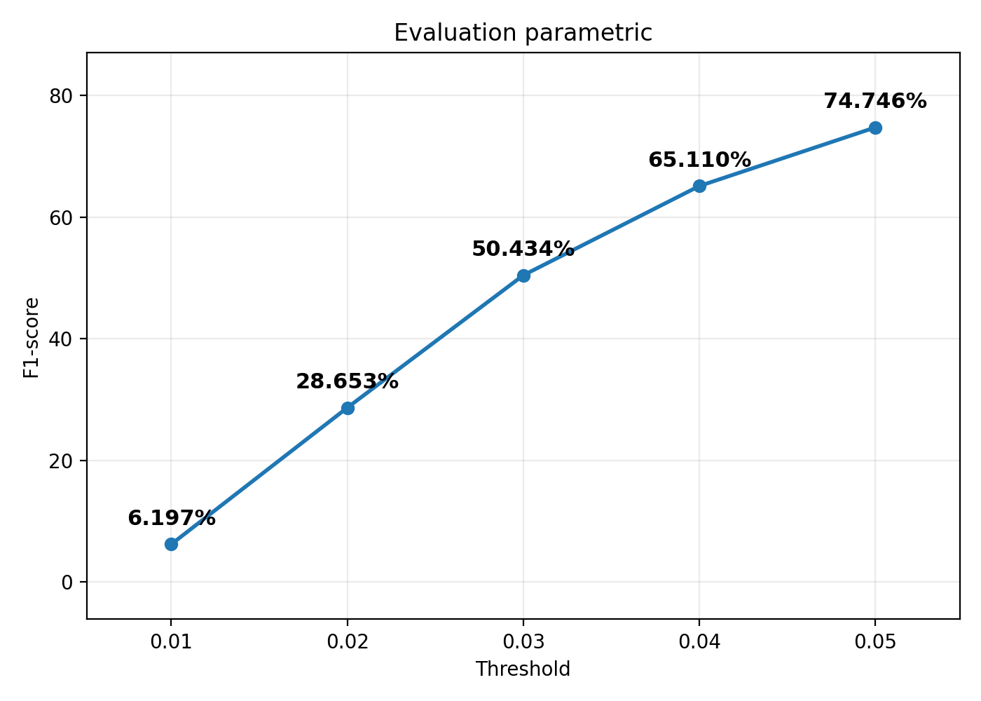
My parametric model, using four surface patches and 1,000 predicted points, achieves an average F1@0.05 score of 74.746% on the test set. The plot shows the average F1 scores at different distance thresholds. The score increases from 6.197% at 0.01 to 74.746% at 0.05, indicating that the predictions approximate the overall geometry but still contain positional errors that become apparent under stricter distance thresholds.
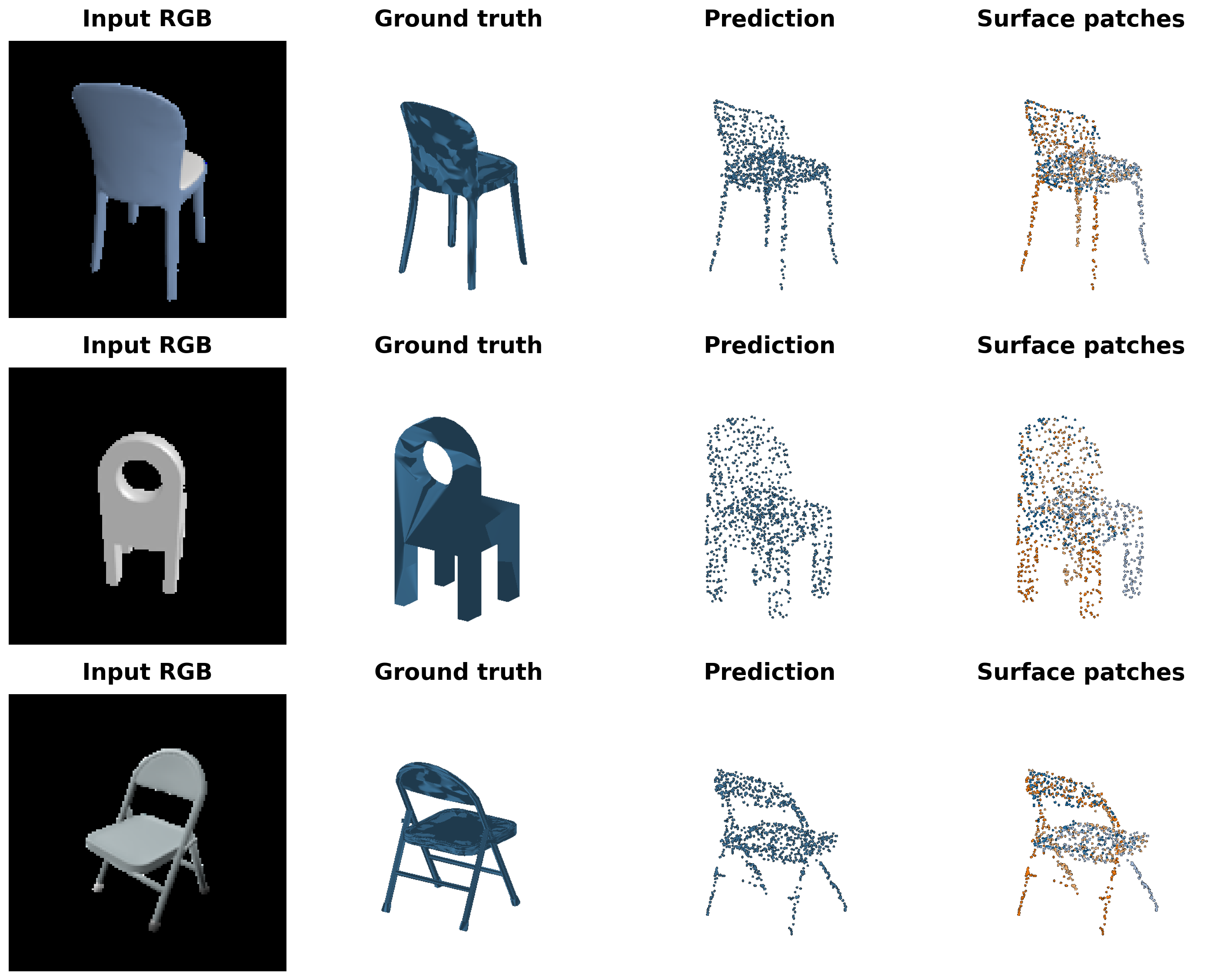
Qualitative results on three test examples. From left to right: the input RGB image, the ground-truth mesh, the predicted point cloud, and the same prediction colored by surface patch. The model captures the main chair structures, including the backrests, seats, and legs, but misses some geometric details. The hole in the second chair’s backrest is not clearly recovered, and the thin supporting bars of the folding chair are incompletely represented.
Each color identifies points generated by one of the four patch decoders; it does not indicate reconstruction error or a predefined semantic part. Different patch colors are interspersed across the backrests and seats, showing that multiple patches contribute to these regions rather than forming a clean separation into chair components. The patches jointly represent the overall shape, but connectivity between them is not explicitly enforced.
3.3 Extended dataset for training (10 points)
The model checkpoint for this task is cps/checkpoint_point_1000_3c.pth, cps/checkpoint_point_1000.pth.
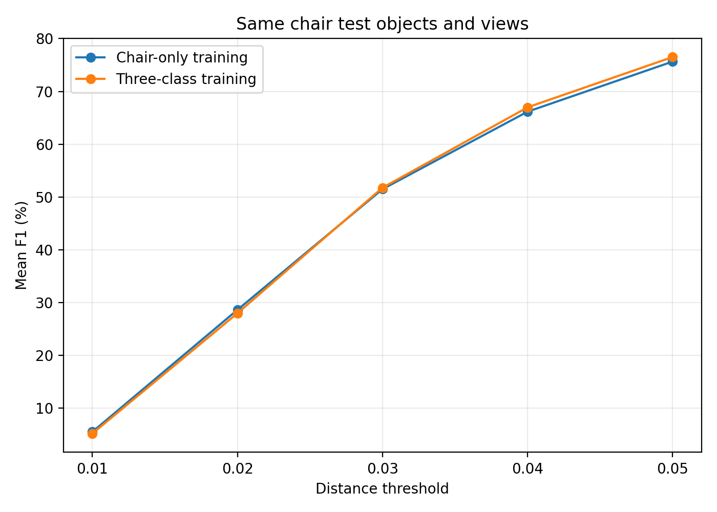
I compare the chair-only and three-class models on the same 678 chair test objects, using identical input views and ground-truth point samples. Both models predict 1,000 points. Their F1 curves are close: the chair-only model performs slightly better at the stricter thresholds of 0.01 and 0.02, while the three-class model achieves slightly higher scores at 0.04 and 0.05. Thus, training jointly on chairs, cars, and airplanes preserves comparable chair reconstruction performance, with a modest improvement at the larger distance thresholds in this run. The results do not show a uniform advantage across all thresholds.
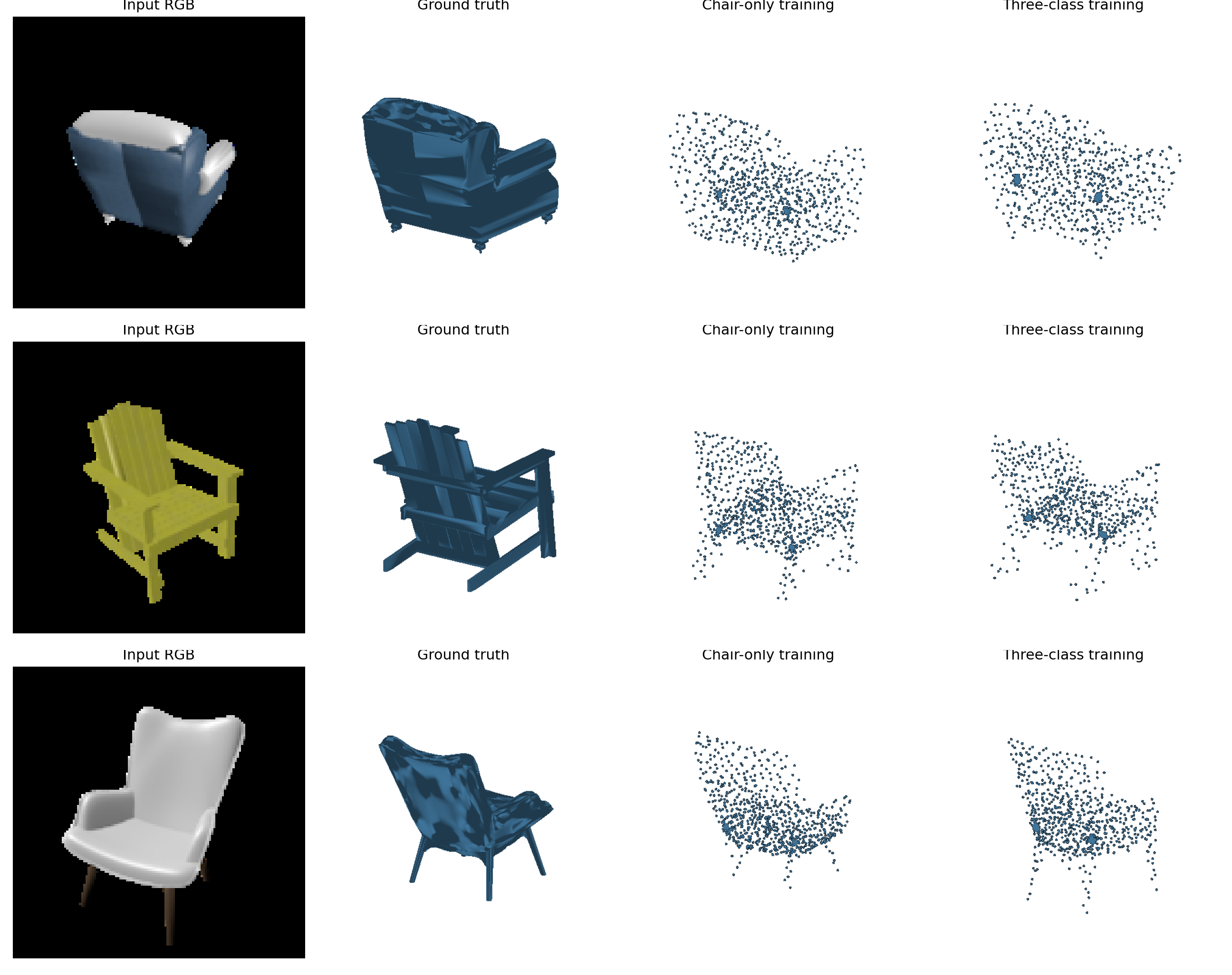
Qualitative comparison on three shared chair test examples. From left to right: the input RGB image, the ground-truth mesh, the chair-only prediction, and the three-class prediction. Both models recover recognizable seat and backrest structures across different chair styles, but thin legs, armrests, and individual slats remain incompletely represented. The three-class model changes the distribution of points over these structures without showing a consistent visual improvement across all three examples. This is consistent with the small differences between their average F1 curves: broader category training retains chair reconstruction ability, but does not resolve all fine-detail errors.
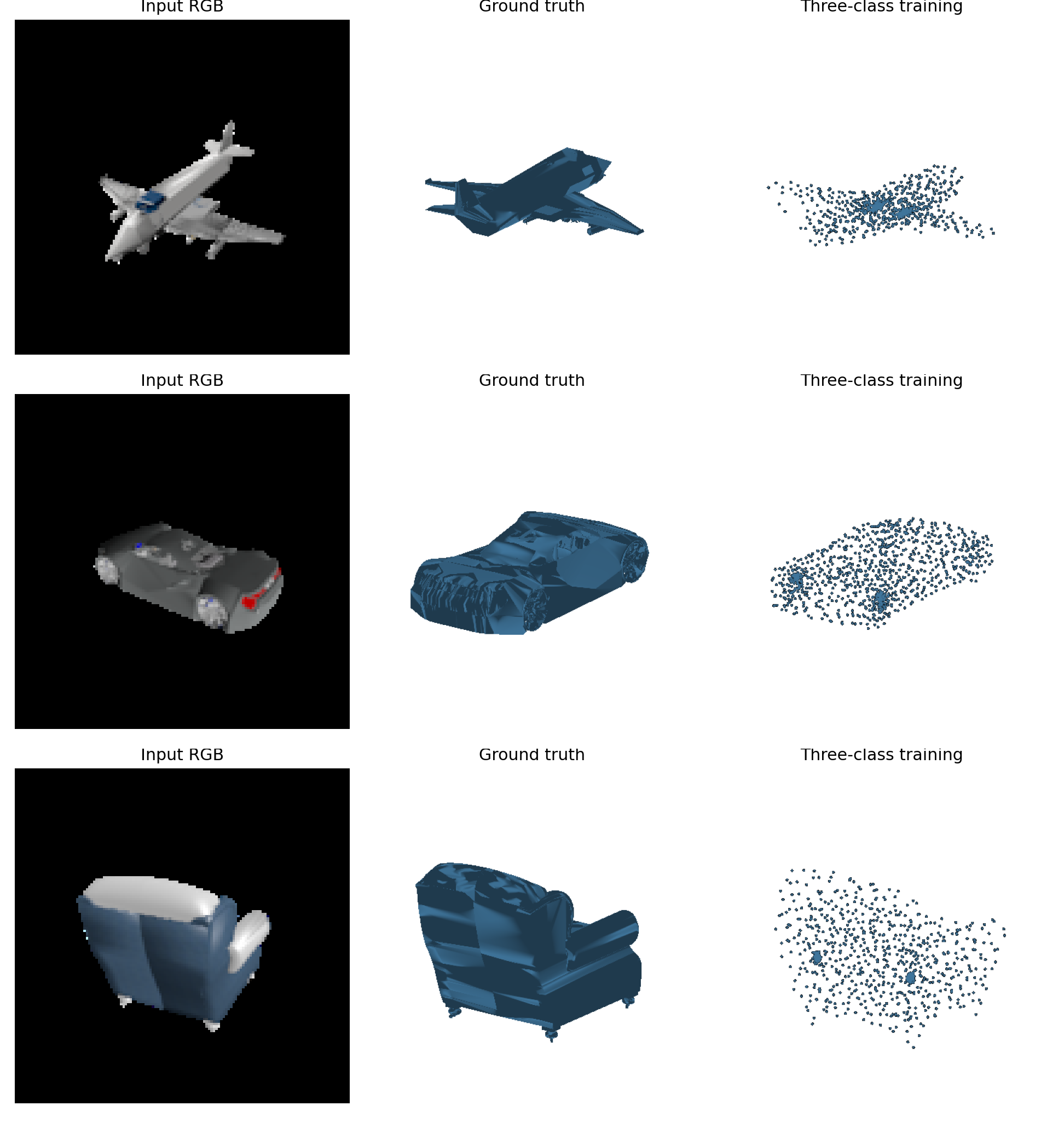
Reconstructions from the model trained jointly on airplanes, cars, and chairs. Each row shows the input image, the ground-truth mesh, and the predicted point cloud. The model produces distinct category-dependent shapes, including an airplane-like fuselage and wings, an elongated car body, and a chair-like seat and backrest. However, fine structures such as aircraft components, wheel geometry, and chair supports are only coarsely represented.
These examples demonstrate that a single shared model can reconstruct multiple object categories without changing its output representation. Together with the matched-chair evaluation, they suggest that the model accommodates a broader range of shapes while maintaining similar chair performance. Learning shared geometric features is one possible explanation, but this experiment does not isolate that mechanism from differences in training data size and sample exposure.
Quantitative Comparison on Matched Chair Examples
Both models are evaluated on the same 678 chair test objects using identical input views and the same 1,000 ground-truth point samples per object. Each model predicts 1,000 points.
| Training data |
F1@0.05 on matched chair examples |
| Chair only |
75.656% |
| Chair + car + plane |
76.513% |
| Difference (three-class − chair-only) |
+0.857 percentage points |
Three-class training produces a modest improvement in chair reconstruction at the 0.05 distance threshold. However, the improvement is not consistent across thresholds: the chair-only model performs slightly better at 0.01 and 0.02, while the three-class model performs better at 0.03–0.05. These results suggest that training on additional categories preserves chair reconstruction performance and slightly improves accuracy under more tolerant distance thresholds in this experiment. Without repeated training runs, this small difference should not be interpreted as a statistically established advantage.
Performance Across Categories
The three-class model achieves higher F1@0.05 scores on cars and planes than on chairs in this evaluation. The overall score is an average over all 1,451 test objects, weighted by the number of objects in each category. It should not be compared directly with the chair-only model’s chair test score because the evaluated category composition differs. The matched-chair comparison above isolates the evaluation to the same objects and views.