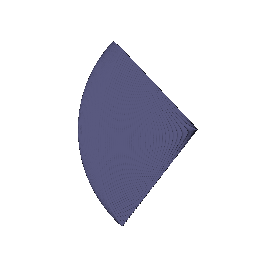
Box center (rounded to 1/100): (0.25, 0.25, 0.00) Box side lengths (rounded to 1/100): (2.01, 1.50, 1.50) (Initial, pre-optimization guess in train_box.yaml: center = (0, 0, 0), side_lengths = (1.5, 1.5, 1.5))
Before vs. after optimization
Rendered at the 4 training camera poses, compared against the actual ground-truth training images.
Before training (cam 0)After training (cam 0)
Before training (cam 1)After training (cam 1)
Before training (cam 2)After training (cam 2)
Before training (cam 3)After training (cam 3)
3. Optimizing a Neural Radiance Field (NeRF)
NeRF on lego, 128×128, position-only (mine)NeRF on lego (TA reference)
4. NeRF Extras
4.1 View Dependence
With view dependence (128×128)Without view dependence (128×128)
The difference between the with- and without-view-dependence renders is very minimal at 128×128 and hard to tell apart by eye. The effect only shows up when looking directly at predicted values instead of the rendered image: querying the model at one fixed 3D point with 6 different viewing directions gives identical density every time, but the predicted color shifts slightly across directions (blue channel ranged from about 0.79 to 0.93). So the model did learn some view-dependence, it is just too subtle here to notice in the final render. This also raises an overfitting risk, since a model free to vary color by direction could be fitting noise in the small set of training camera angles instead of learning real reflectance, and an effect that only shows up when probing specific points rather than in normal renders is consistent with that.
4.2 Coarse/Fine Sampling
Coarse/fine NeRF on lego, 128×128
Coarse/fine sampling runs two networks per step, so it is about half the speed of the single-network baseline (13 to 17 it/s versus 29). Despite the extra cost, it reaches a similar final loss (about 0.005 to 0.009, comparable to the baseline) and shows minimal improvement at this resolution.
4.3 VolSDF
Best result: alpha=10, beta=0.15, eikonal_weight=0.02
Color (mine)Color (TA reference)
Geometry (mine)Geometry (TA reference)
Hyperparameter sweep
alpha
beta
eikonal_weight
Color
Geometry
10 (default)
0.05 (default)
0.02 (default)
5
0.05
0.02
20
0.05
0.02
10
0.01
0.02
10
0.08
0.02
10
0.15
0.02
10
0.2
0.02
10
0.3
0.02
10
0.05
0.1
Alpha is the maximum density the surface can reach, how opaque it gets deep inside the object. Beta controls how sharp the transition from empty space to solid surface is: small beta gives a thin, wall-like transition right at the surface, large beta spreads that transition over a wider band, giving a softer, foggier edge.
High beta biases the learned surface toward being soft and smoothed out, blurring away fine detail. Low beta biases it toward sharp detail, but makes the density very sensitive to small errors in the predicted distance near the surface, which shows up as floaters. We saw this directly: beta=0.01 produced floaters across the whole ground plane, and beta=0.3 smoothed the object into a shapeless blob.
Easier at high beta, since the density transition is spread over a wider region, giving smoother and less noisy gradients for the photometric loss. Low beta concentrates density into a thin spike, which gives sparse, high-variance gradients and makes optimization less stable.
Neither extreme works well. Low beta gives noisy floaters away from the true surface, and high beta smooths away the real surface detail. An accurate surface needs a middle value, sharp enough to keep detail but not so sharp that noise turns into floaters, which matches what the sweep showed.
beta=0.15 (alpha=10, eikonal_weight=0.02, all else default) gave the cleanest geometry with minimal floaters while keeping sharp detail, better than both the noisier low-beta runs and the blobbier beta=0.2/0.3 runs. Raising eikonal_weight alone to 0.1 did not help and produced more floaters, and changing alpha alone (5 or 20) did not fix the floater issue either.
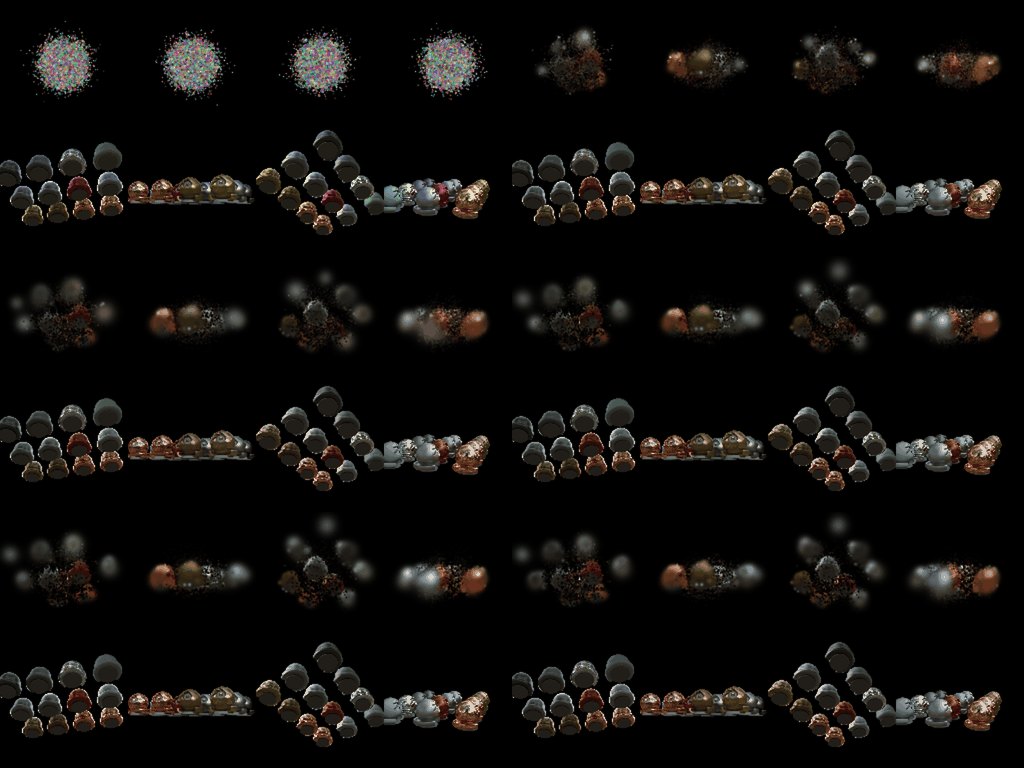
Learning rates: means = 0.0005, opacities/scales/colours = 0.01 Iterations: 1000 Mean PSNR: 29.511 Mean SSIM: 0.940
Training progress (top: predicted, bottom: ground truth)Final renders on training views
7. Extensions
7.1 Rendering Using Spherical Harmonics
Without SH (DC only, question 5.5)With SH (question 7.1)
Side-by-side comparisons (same view)
Without SHWith SH
Without SHWith SH
Without SHWith SH
Frame 0: SH version shows noticeably richer, sharper detail on the armrests and backrest, visible wood grain and a clearer floral pattern. The non-SH version looks flatter and softer in the same areas.
Frame 8: This frame is a near-degenerate top-down viewing angle where both renders show streaking artifacts from the camera path. The streaking dominates at this angle, so any color difference between SH and non-SH is hard to judge reliably here.
Frame 16: Same pattern as frame 0, the SH render has more saturated, defined gold trim and floral texture, while the non-SH version looks washed out by comparison.
Together, the three frames give a good sense of how SH affects shading: it adds visible depth and shadowing to the texture and trim that the flat DC-only colour misses.
7.2 Training On a Harder Scene
Dataset: materials (NeRF synthetic). All runs below use isotropic Gaussians unless noted, init_type="random".
Baseline (question 6.2 setup, applied to this dataset)
Learning rates: means = 0.0005, opacities/scales/colours = 0.01 Iterations: 1000, num_points = 10000 Mean PSNR: 18.124 Mean SSIM: 0.671
Training progressFinal renders
Ablations at 10,000 points, 1000 iterations
Variant
PSNR
SSIM
Progress GIF
Final renders GIF
baseline
18.124
0.671
anisotropic
18.807
0.668
SSIM loss
17.923
0.679
anisotropic + SSIM loss
18.140
0.679
anisotropic + SSIM loss + 5000 itrs
18.222
0.710
30,000 points, 5000 iterations
Variant
PSNR
SSIM
Progress GIF
Final renders GIF
baseline
19.565
0.717
anisotropic
19.426
0.715
SSIM loss
18.420
0.710
anisotropic + SSIM loss
18.669
0.718
There are two different "best" results depending on the metric. The plain baseline at 30,000 points and 5000 iterations got the best PSNR (19.565), while adding anisotropic Gaussians and SSIM loss on top of that got the best SSIM (0.718) but a slightly lower PSNR (18.669). So raw pixel accuracy and structural similarity do not agree on the same model here.
The main modification versus the 6.2 baseline was increasing the number of points from 10,000 to 30,000 and training for 5000 iterations instead of 1000, since all the ablations at 10,000 points plateaued around the same PSNR and SSIM regardless of loss function or Gaussian shape. This pointed to a capacity problem: random sphere initialization scattered across a scene with several separate objects likely does not have enough Gaussians to cover the scene, no matter how well the existing points are placed. Moving to 30,000 points confirmed this, giving a clear jump in both PSNR and SSIM over every 10,000-point variant. Anisotropic Gaussians and SSIM loss were kept from the earlier ablations since they gave the best SSIM when combined, even though they did not improve PSNR over the plain 30,000-point baseline.