
Name: Tashvik Dhamija (tdhamija)


Trained for 6000 iterations. Architecture: ResNet18 encoder → Linear(512, 64) → reshape to (1, 4, 4, 4) → 3x ConvTranspose3d (4³ → 8³ → 16³ → 32³).


Avg F1@0.05 = 43.7%
Trained for 3000 iterations, n_points = 1000. Architecture: ResNet18 encoder → Linear(512, 1024) → ReLU → Linear(1024, 1024) → ReLU → Linear(1024, n_points * 3).


Avg F1@0.05 = 77.7% (n_points = 1000)
Trained for 3000 iterations. Architecture: ResNet18 encoder → Linear(512, 1024) → ReLU → Linear(1024, 1024) → ReLU → Linear(1024, n_verts * 3) vertex offsets, applied to an icosphere (subdivision level 4) initial mesh.


Avg F1@0.05 = 70.5%
| Representation | Avg F1@0.05 |
|---|---|
| Voxel grid | 43.7% |
| Point cloud | 77.7% |
| Mesh | 70.5% |
The voxel grid performs worst because the model has to learn the spatial dependencies between neighboring voxels through the convolutional decoder, which is a harder relationship to learn. The coarse 32³ grid resolution adds to this problem, since fine details like thin chair legs are easy to lose entirely at that resolution.
The mesh performs better, but deforming a fixed topology icosphere with a fixed number of triangle primitives can force artifacts. The mesh has to bend a constrained set of triangles into shapes they are not naturally suited for, which shows up as jagged, distorted geometry.
The point cloud shows the best understanding of shape overall, but with a fixed n_points budget, the predicted points end up dense in the high confidence central body of the chair, while fewer points populate the less certain extremities, such as the backrest and the legs.
Varying n_points (the number of points the point-cloud decoder predicts and that chamfer loss is computed over) for the point cloud model, keeping all other hyperparameters fixed. Each variant (500, 1000, 1500) was trained for 3000 iterations with the same architecture as 2.2.


F1@0.05 increases monotonically with n_points (70.8% → 77.7% → 81.6%). A denser predicted point cloud gives finer-grained coverage of the true surface, which directly improves the precision/recall computation at a fixed distance threshold. The tradeoff is compute and memory cost per sample (and diminishing returns are expected eventually), but within this range, more points reliably helps.
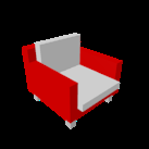
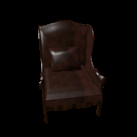
To understand what the learned image feature represents, I encode two different test images independently with the ResNet18 encoder, then linearly interpolate between their two 512-d feature vectors (t = 0, 0.25, 0.5, 0.75, 1) and decode each interpolated feature. If the decoder learned a smooth, generalizable shape space (rather than memorizing specific outputs), the in-between predictions should look like coherent, plausible intermediate chairs rather than incoherent noise.


The voxel model shows the clearest, smoothest morph between the two endpoint shapes across all 5 steps. Point cloud interpolation shows visible but more subtle shape change (point density/spread shifting gradually). Mesh interpolation also shows gradual change in size/shape, though the predicted mesh surfaces are consistently jagged and self-intersecting regardless of interpolation step, reflecting the same fixed topology constraint discussed in 2.3.
Trained for 2000 iterations. Architecture: ResNet18 encoder → two-stage FiLM-conditioned coordinate MLP → Linear(256, 1) occupancy logit, queried at a fixed 32³ grid of points in (-1,1)³.
An implicit decoder takes a 3D coordinate and the image feature as input and outputs an occupancy value at that point, instead of predicting a whole fixed-size grid in one forward pass. The image feature conditions the coordinate pathway via two stacked FiLM (scale and shift) layers. At inference, the network is queried at the full grid to reconstruct the occupancy grid, which is then converted to a mesh via marching cubes, the same as the voxel grid pipeline in 2.1.
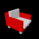

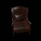

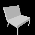
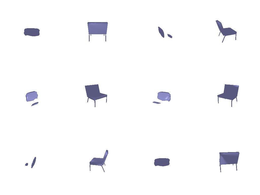
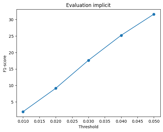
Avg F1@0.05 = 31.6%
Trained for 2000 iterations. Architecture: ResNet18 encoder → two-stage FiLM-conditioned coordinate MLP → Linear(256, 3) output point, applied to a fixed set of n_points sampled on (-1,1)².
A parametric decoder maps sampled 2D points on a fixed (-1,1)² domain to 3D points, instead of regressing all output points directly from the image feature alone as the point cloud decoder in 2.2 does. The image feature conditions the 2D coordinate pathway via the same two-stage FiLM (scale and shift) design used in 3.1, with a final linear layer outputting 3D coordinates instead of an occupancy value.



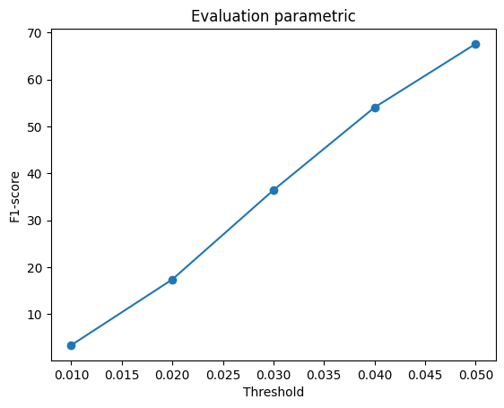
Avg F1@0.05 = 67.6%