1. Multi-View Data Preprocessing
1.2. Depth Unprojection


1.3. Camera and Depth Canonicalization
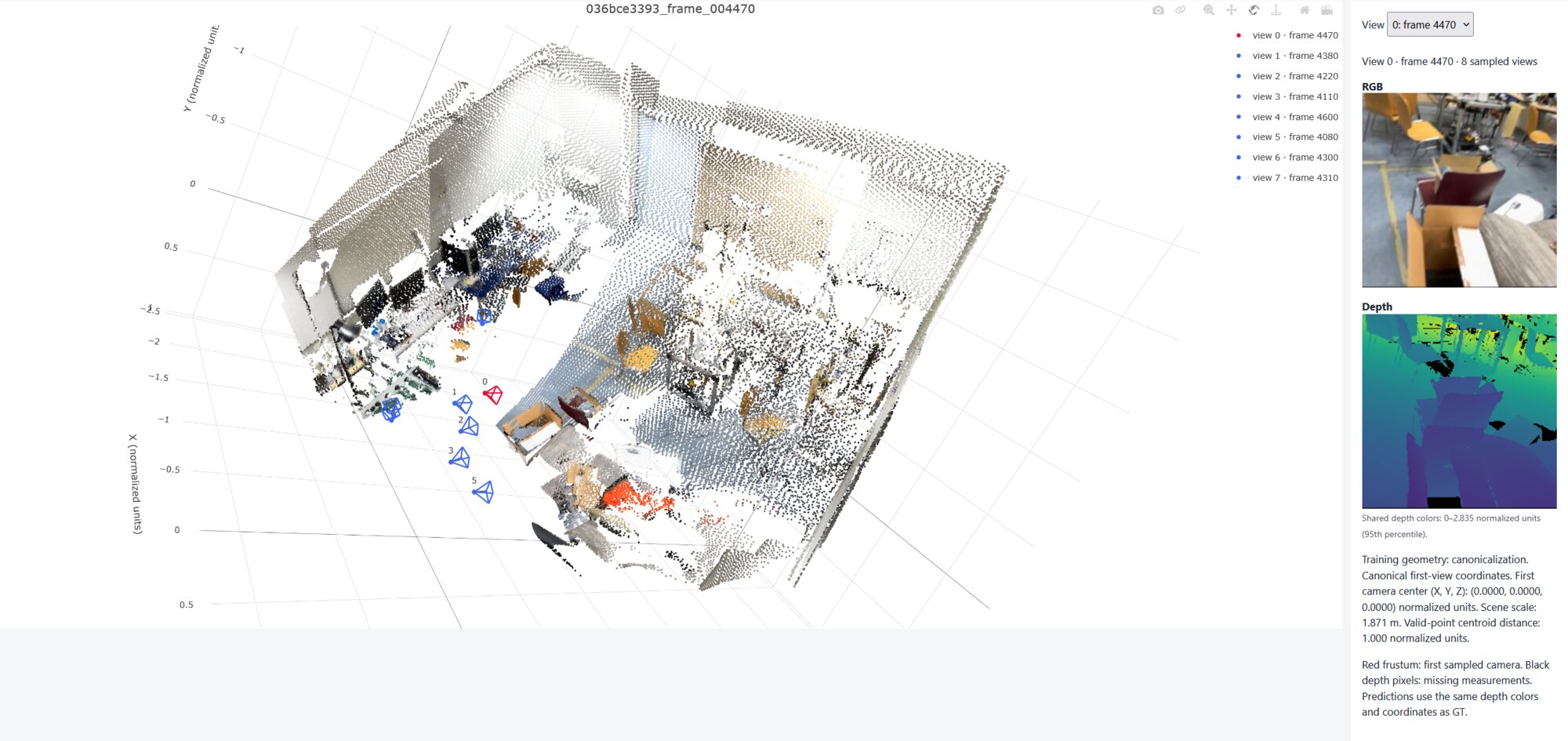
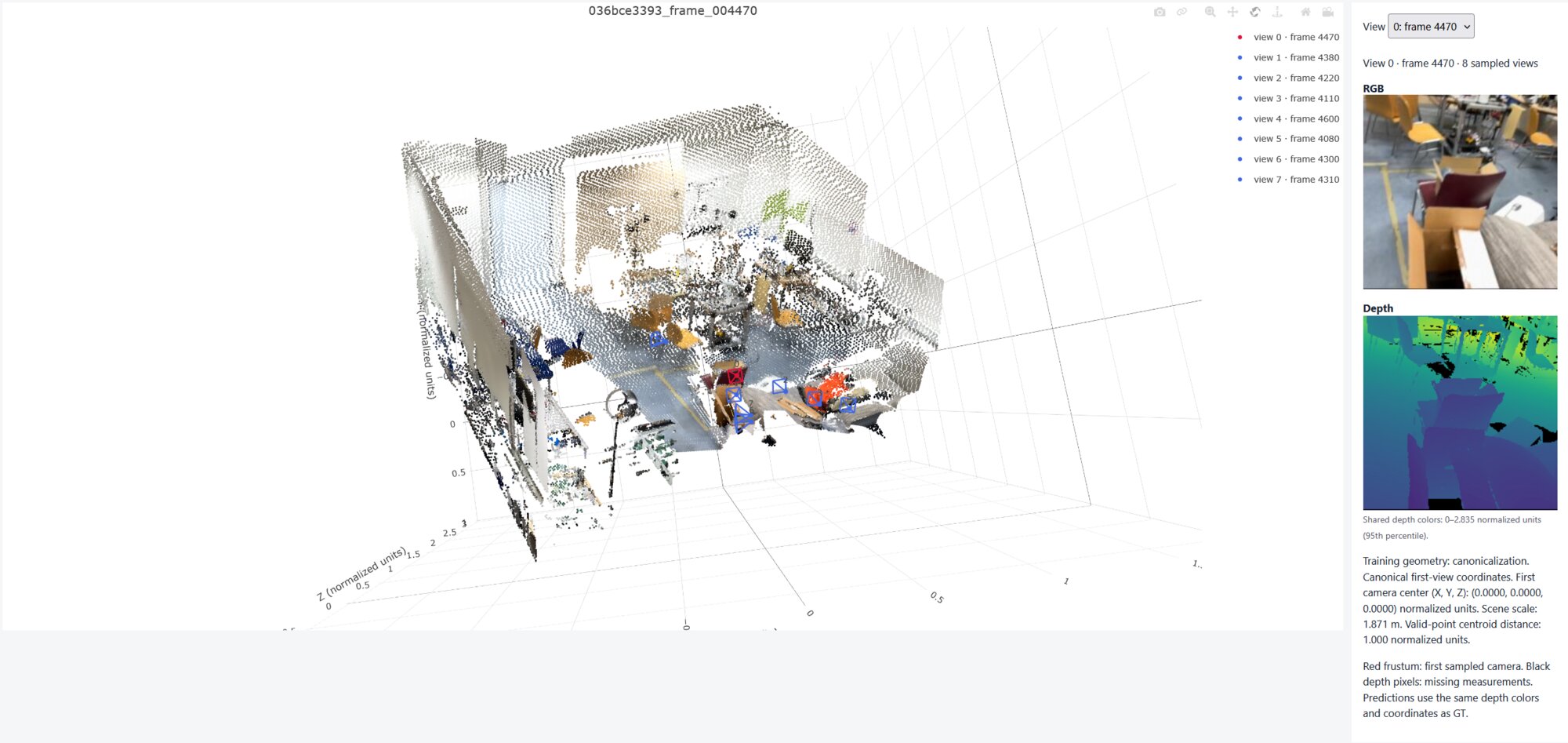
1.7. Final Check
check_data.py output:
{
  "split": "train",
  "dataset_samples": 224,
  "checked_samples": 4,
  "samples": [
    {
      "sequence_name": "e050c15a8d_frame_007080",
      "views": 8,
      "resolution": 224,
      "valid_depth_fraction": 0.9733812212944031,
      "max_reprojection_error_px": 0.0001089862416847609,
      "max_ray_reprojection_error_px": 9.423537994734943e-05,
      "centroid_distance": 0.9999999403953552
    },
    {
      "sequence_name": "5f99900f09_frame_002820",
      "views": 8,
      "resolution": 224,
      "valid_depth_fraction": 0.9858846664428711,
      "max_reprojection_error_px": 0.00013037114695180207,
      "max_ray_reprojection_error_px": 0.0001258271950064227,
      "centroid_distance": 1.0
    },
    {
      "sequence_name": "47b37eb6f9_frame_002720",
      "views": 8,
      "resolution": 224,
      "valid_depth_fraction": 0.9563461542129517,
      "max_reprojection_error_px": 9.770392352947965e-05,
      "max_ray_reprojection_error_px": 9.770392352947965e-05,
      "centroid_distance": 1.0
    },
    {
      "sequence_name": "4c5c60fa76_frame_006690",
      "views": 8,
      "resolution": 224,
      "valid_depth_fraction": 0.7481689453125,
      "max_reprojection_error_px": 0.00010796334390761331,
      "max_ray_reprojection_error_px": 0.00010322615707991645,
      "centroid_distance": 1.0
    }
  ],
  "batch_shapes": {
    "rgb": [
      2,
      8,
      3,
      224,
      224
    ],
    "depth": [
      2,
      8,
      1,
      224,
      224
    ],
    "depth_valid": [
      2,
      8,
      1,
      224,
      224
    ],
    "K": [
      2,
      8,
      3,
      3
    ],
    "frame_numbers": [
      2,
      8
    ],
    "T_world_from_camera": [
      2,
      8,
      4,
      4
    ],
    "original_world_from_reference": [
      2,
      4,
      4
    ],
    "scene_scale": [
      2
    ],
    "points_world": [
      2,
      8,
      3,
      224,
      224
    ],
    "ray_origins": [
      2,
      8,
      3,
      224,
      224
    ],
    "ray_directions": [
      2,
      8,
      3,
      224,
      224
    ],
    "plucker": [
      2,
      8,
      6,
      224,
      224
    ]
  }
}
Full Render


Briefly explain canonicalization, world-space ray directions and the Plücker moment.
- Canonicalization: In order to be able to unproject points from different images (with different viewpoints) into the same 3D scene, we first need to make sure that all images are in a consistent scale and coordinate frame (our canonical frame). In our case, we take our coordinate frame as the coordinate frame of the first camera (i.e. index 0), then choose our scene scale such that the centroid of valid points in the first camera's frame will be of distance 1 from our canonical frame's origin. Canonicalization, then, is the process of transforming and rescaling the other images' frames and points into our new canonical frame & scale. To obtain their transformations relative to our new canonical frame's origin, we multiply their camera-to-world poses by the inverse of the first camera's camera-to-world pose; this, as well as the images' depth measurements, are then divided by the scene scale to make the scale match.
- World-space ray directions: Each pixel in a depth image corresponds to a 3D point at a certain distance from the camera, in a particular direction. Said direction can be represented as a ray corresponding to that specific pixel, such that the process of unprojecting the depth pixel into the original 3D point would require only traveling a certain distance along that ray [the depth] and placing the point. Since we are working with multiple views, however, we want our output 3D points to be in the world frame; then the appropriate camera-to-world rotation must be applied to the camera-frame ray direction to map it into a world-frame ray direction. Notably, the ray direction only represents the direction of a ray, not the starting point/origin of the ray.
- Plücker moment: As mentioned, a 3D ray can be represented by two 3-vectors, a direction $d$ and a starting point/origin $o$. In terms of geometry, the Plucker moment of a ray is a vector that is normal to the plane spanned by the ray's aforementioned direction and origin vectors (i.e. the plane through the world origin and the ray), which can be computed via the cross product $m=o\times d$. Notably, any given 3D ray is the unique ray corresponding to a direction-moment pair ($d,m$); as such, a Plucker representation is an alternate parametrization of a ray that, notably, is less susceptible to causing a network to learn associations based on the absolute value of the origin $o$, and is unique [unlike the ($d,o$) direction-origin representation, which is only unique up to translations of the origin along the ray].
2. Novel-View Synthesis with Mini-LVSM

2.2. Training and Evaluation
Training Settings
All settings were the same as in the assignment repository.
{
  "data_config": "configs/scannetpp/iphone/data.json",
  "data_overrides": {
    "batch_size": 4,
    "eval_num_frames": 32
  },
  "model": {
    "patch_size": 8,
    "d_model": 384,
    "n_layers": 8,
    "head_dim": 64,
    "mlp_ratio": 4.0,
    "use_qk_norm": true
  },
  "loss": {},
  "training": {
    "epochs": 100,
    "learning_rate": 0.0002,
    "weight_decay": 0.05,
    "betas": [0.9, 0.95],
    "warmup_steps": 200,
    "grad_clip": 1.0,
    "amp": true,
    "vis_every": 5,
    "output_dir": "outputs/lvsm"
  },
  "num_source_views": 2
}
Training Curves

Training Visualizations
val_epoch000.jpg:

val_epoch050.jpg:

val_epoch095.jpg:

Ablation Visualizations
S=1
S1_correct.jpg:

S1_none.jpg:

S1_shuffled.jpg:

S=2
S2_correct.jpg:
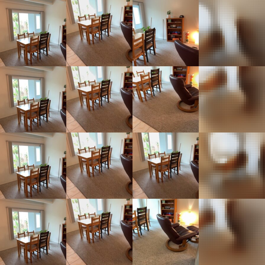
S2_none.jpg:
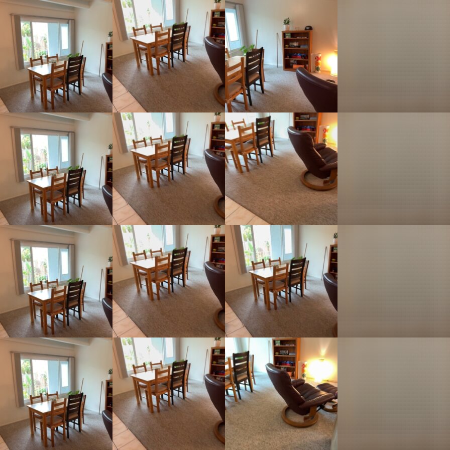
S2_shuffled.jpg:

S=4
S4_correct.jpg:
S4_none.jpg:
S4_shuffled.jpg:

Metrics
Validation PSNR:
correct |
shuffled |
none |
|
|---|---|---|---|
S=1 |
15.196 | 11.772 | 12.463 |
S=2 |
16.121 | 11.406 | 12.426 |
S=4 |
16.829 | 11.518 | 12.410 |
Validation SSIM:
correct |
shuffled |
none |
|
|---|---|---|---|
S=1 |
0.557 | 0.485 | 0.531 |
S=2 |
0.558 | 0.469 | 0.529 |
S=4 |
0.574 | 0.471 | 0.538 |
Discussion
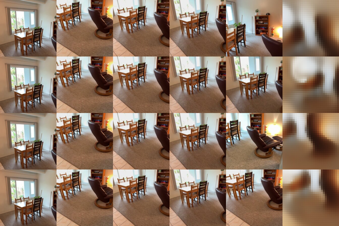
For the source views comparison, the shuffled predictions don't appear to look any worse than the correct predictions; the only difference is that the shuffled predictions don't match the viewpoint of the target image, unlike the correct predictions. This is fairly expected, as the shuffled rays are a valid set of rays, just for a different view than the target image is taken from. In contrast, the none predictions are all identical within their respective # source views conditions, i.e. all of the S=1 none predictions look identical, the S=2 none predictions, look identical, etc. This is, again, expected, as we are feeding the same set of views [i.e. all zeros] to each of them. Interestingly, though, the none predictions are not a constant color, and although it's difficult to tell, they do appear to differ between the different # source view conditions as well. It's possible that although the input rays are the same for all patches (i.e. all zeroes), the network is able to extract some kind of underlying pattern between patch index and output RGB that comes out even when rays are all zero, hence why the outputs are some kind of muddled gradients.
(For the # views comparison, I am talking exclusively about the correct renders.) In terms of number of views, the big difference is in which objects are/aren't visible in the source views and, consequently, are/aren't represented in the final prediction. For the S=1 condition, for instance, the only source view has the right-side armchair mostly out of sight, and only half of the bookshelf in view. As such, all predictions only feature a very thin bookshelf (likely corresponding to its left half only) and no chair at all, whereas in the S=4 condition (with more of the bookshelf and chair in view), the bookshelf and chair are, in fact represented. Similar observations can be made with regards to S=2, where the source views lack both the lamp and the right half of the lamp and, which are thus also missing in the S=2 renders, whereas they appear in the S=4 renders that do take input views with the lamp and right half of the chair. Beyond these differences, however, I did not notice a big difference in the rendering quality between any of the three conditions (S=1,S=2,S=4) for the objects that did appear in all three conditions, namely the dining table and chairs.
2.3. Bonus: Analysis and Exploration
For this section, I added an SSIM loss term to the loss function, i.e. $loss=MSE+\lambda\cdot SSIM$, in order to see what effect introducing an additional term to the loss function might have on the model's predictions. In my setup, I used $\lambda=0.01$ as a guess; in practice, the SSIM loss term (multiplied by $\lambda$) ended up being ~20% of the MSE loss term.
Training Curve
All training settings were kept the same as in Q2.2.

Visualizations
(All visualizations are on the correct setting.)
S=1, without SSIM:
S=1, with SSIM:

S=2, without SSIM:
S=2, with SSIM:

S=4, without SSIM:
S=4, with SSIM:

Although the differences are relatively minor, it seems like the addition of the SSIM term results in the prediction being slightly sharpened and/or eroded (at least as far as objects go) relative to the no-SSIM prediction. This is most clearly visible in the first and last images of the S=1 setting, where the chair and bookshelf appear slightly smaller and more well-defined in the SSIM predictions than the non-SSIM predictions; this is maybe also true for the first and second images in the S=4 setting, although I'm less sure about those two.
The SSIM predictions also maybe seem to be slightly brighter and more colorful (or maybe just higher contrast?) than the non-SSIM predictions, as seen in the third image of the S=2 and the second image of the S=4 setting, for both of which the SSIM window and table appear slightly brighter and more colorful, respectively, than in the corresponding non-SSIM predictions.
Metrics:
Validation PSNR:
correct w/ SSIM |
correct w/o SSIM |
shuffled w/ SSIM |
shuffled w/o SSIM |
none w/ SSIM |
none w/o SSIM |
|
|---|---|---|---|---|---|---|
S=1 |
15.104 | 15.196 | 11.799 | 11.772 | 12.401 | 12.463 |
S=2 |
16.046 | 16.121 | 11.475 | 11.406 | 12.381 | 12.426 |
S=4 |
16.690 | 16.829 | 11.565 | 11.518 | 12.409 | 12.410 |
Validation SSIM:
correct w/ SSIM |
correct w/o SSIM |
shuffled w/ SSIM |
shuffled w/o SSIM |
none w/ SSIM |
none w/o SSIM |
|
|---|---|---|---|---|---|---|
S=1 |
0.569 | 0.557 | 0.498 | 0.485 | 0.534 | 0.531 |
S=2 |
0.573 | 0.558 | 0.484 | 0.469 | 0.533 | 0.529 |
S=4 |
0.588 | 0.574 | 0.486 | 0.471 | 0.543 | 0.538 |
Looking mainly at the metrics for the correct setting, we see that the no-SSIM model has slightly higher PSNR across all three # source view settings (S=1,2,4), whereas the SSIM model has slightly higher SSIM. It's not too surprising that the SSIM model has better SSIM values (since SSIM is directly represented in the loss term), but the fact that the no-SSIM model outperforms on PSNR seems to indicate that there's some kind of PSNR-SSIM tradeoff in play. That said, our predictions are pretty low-quality, meaning both models have a long way to go in terms of improvement; as such, it's not guaranteed that this kind of same tradeoff would still hold when evaluated on better models with higher-quality predictions.
Beyond the correct setting, the SSIM model beats the no-SSIM model in terms of SSIM on the shuffled and none settings and, strangely enough, also does slightly better on the shuffled setting for PSNR. One notable difference between SSIM and PSNR is that PSNR primarily relies on pixel-wise error, whereas SSIM is computed over larger neighborhoods/windows. As such, it could be that the SSIM loss term is inducing some kind of filter over the outputs, as each pixel will now be receiving gradients from the computation of SSIM on neighboring pixels other than themselves. In terms of the observations made regarding the images, this could be the effect of the hypothesized erosion at work, where, on the shuffled settings, the erosion decreases the size of the bookshelf, chair, and table in the image and thus bumps down the pixel-wise error on those regions (which might correspond to more neutral colors, e.g. beige, in the target view).
Overall, although subtle, it does appear that the SSIM term is having some kind of effect on the predictions, as mentioned in my observations regarding the visualizations (as well as the differences in the PSNR & SSIM errors), which may or may not correspond to some kind of filtering effect on the output images. That said, it's difficult to draw conclusions given how blurry and indistinct both models' outputs are -- it's likely that were we to make our models higher-resolution, it could be easier to spot any discrepancies that appear.
3. Multi-View Geometry with Mini-VGGT
3.1. Overfitting
Loss curves:

Visualizations:
View 1 (GT top, predicted bottom):

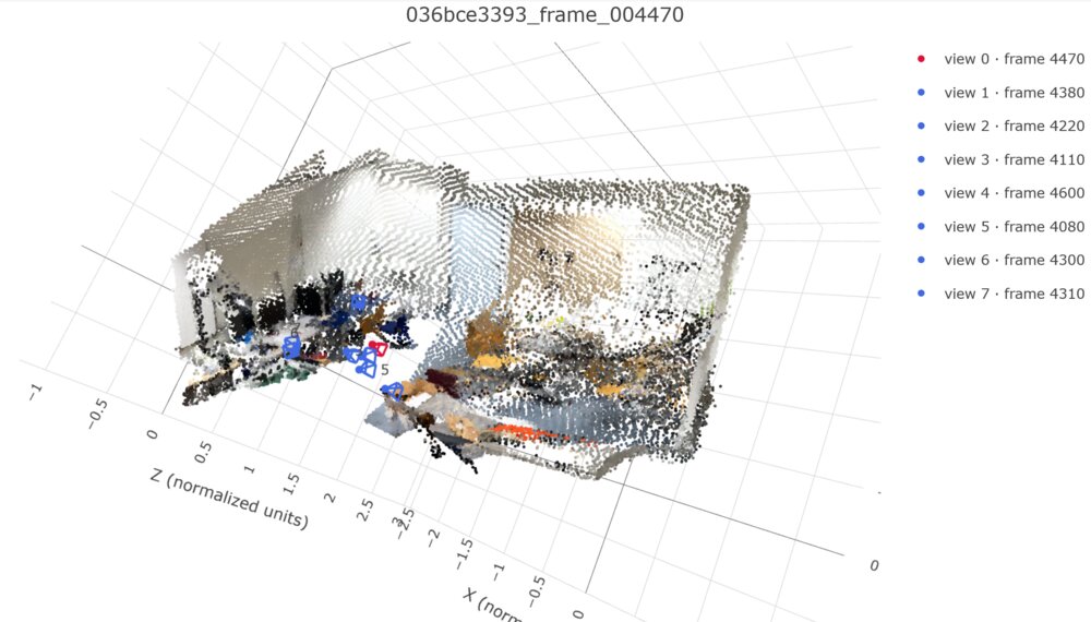
Comparing from a relatively "even" camera angle, our predicted output looks pretty good. It's not quite as sharp as the GT, and the prediction doesn't quite capture some of the smaller elements/details of the scene (e.g. the armrest on the central orange chair, the legs on the table next to it), but overall the geometry looks reasonable and close enough to the GT.
View 2 (GT top, predicted bottom):

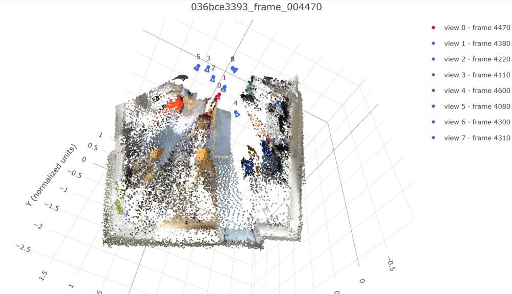
Some of the cracks start to appear from a weird perspective (vertical) not present in the source views, where we see that the predicted geometry seems to suffer from points having been "scattered" or smeared in a direction roughly parallel to the viewing axis, away from the cameras. This is most easily seen in the middle-top-right floating objects in the GT, where the prediction has dispersed these objects into clearly-visible rays.
3.2. Training and Evaluation
Training Settings
All settings are default/the same as in the assignment repository, with the exception of batch size ($16$ [default] $\to8$).
{
  "data_config": "configs/scannetpp/iphone/data.json",
  "data_overrides": {
    "num_views": 8,
    "sampling_range": 32,
    "eval_num_frames": 32,
    "batch_size": 8,
    "num_workers": 8
  },
  "model": {
    "embed_dim": 384,
    "num_heads": 6,
    "num_layers": 8,
    "predict_points": false,
    "encoder_name": "dinov2_vitb14",
    "image_size": 224
  },
  "loss": {
    "camera": 5.0,
    "depth": 1.0
  },
  "training": {
    "epochs": 1000,
    "learning_rate": 0.0006,
    "weight_decay": 0.01,
    "output_dir": "outputs/vggt",
    "overfit_scenes": 1,
    "overfit_steps_per_epoch": 25,
    "min_lr_ratio": 0.05,
    "log_every": 10,
    "warmup_epochs": 10,
    "overfit_epochs": 40,
    "overfit_learning_rate": 0.001
  }
}
Loss curves

Metrics
val |
test |
|
|---|---|---|
| Depth AbsRel | 0.157 | 0.164 |
| Depth δ1 | 0.796 | 0.782 |
| Rotation AUC ($5^\circ$) | 0.173 | 0.174 |
| Rotation AUC ($15^\circ$) | 0.482 | 0.478 |
| Rotation AUC ($30^\circ$) | 0.679 | 0.687 |
| Translation AUC ($5^\circ$) | 0.014 | 0.006 |
| Translation AUC ($15^\circ$) | 0.084 | 0.053 |
| Translation AUC ($30^\circ$) | 0.195 | 0.167 |
| Joint Pose AUC ($5^\circ$) | 0.006 | 0.002 |
| Joint Pose AUC ($15^\circ$) | 0.072 | 0.032 |
| Joint Pose AUC ($30^\circ$) | 0.180 | 0.144 |
Visualizations
Scene 0, view 1 (GT top/predicted bottom):
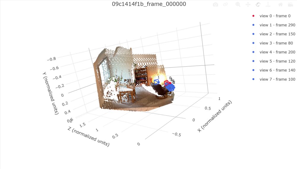
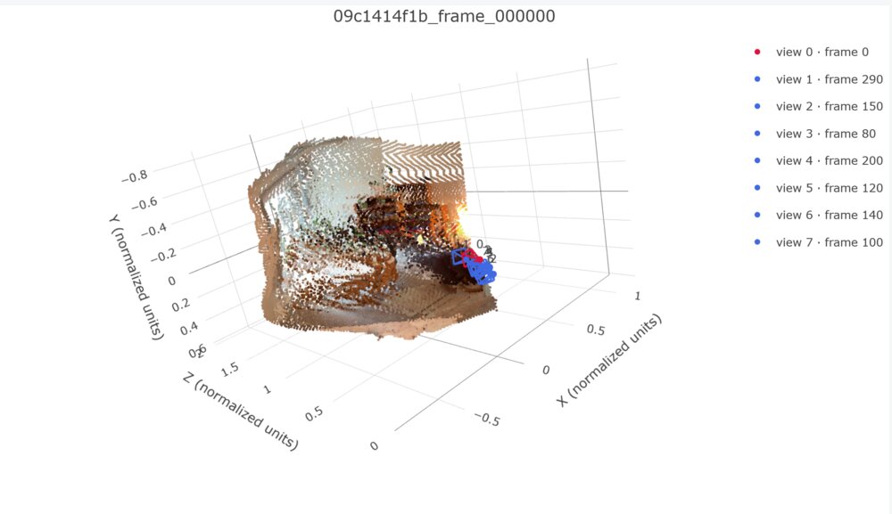
From a view that is almost camera-aligned, but not quite, we can notice some oddities already -- the predicted bookshelf appears to have multiple copies, for instance, and the table geometry is kind of dispersed/scattered (this is a pattern amongst these renderings).
Scene 0, view 2 (GT top/predicted bottom):

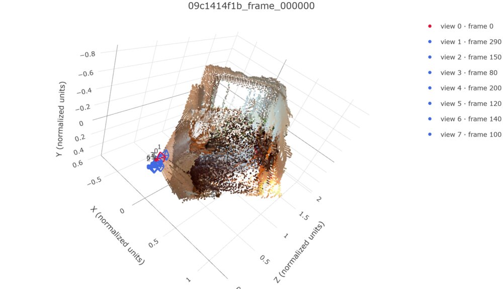
Here, from a view that is further off from the camera, we can see more of the aforementioned scattering in points in the predicted output. Notably, the scattering appears to be in a direction that is roughly parallel to the viewing axes. In theory, we would expect our depth loss to constrain this somewhat; in practice, it's possible that these points could be low confidence, or that our depth loss weight was too low. Adding additional views of the scene from different angles could also help.
Scene 1, view 1 (GT top/predicted bottom):

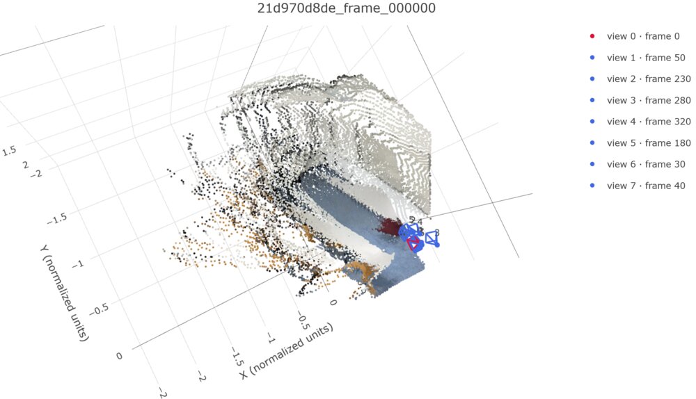
The whiteboard doesn't look too bad, and the predicted chairs in the first row are somewhat distinguishable, but again we see more scattering, plus the chairs in the second row appear to have globbed together.
Scene 1, view 2 (GT top/predicted bottom):

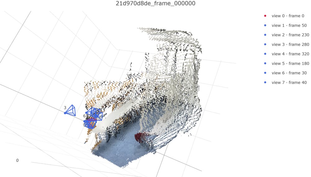
Here, we can see some of the rougher geometry around the whiteboard/wall area, which we would expect to be a planar surface, but isn't in the prediction.
Scene 2, view 1 (GT top/predicted bottom):

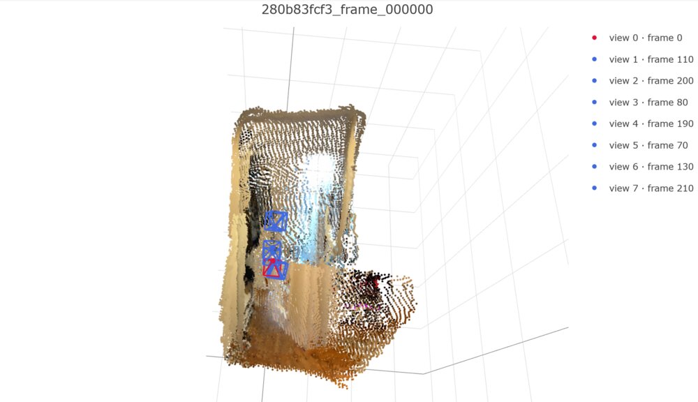
A big misprediction here - the prediction appears to think that the door was half-ajar in the input images, whereas it wasn't (hence the cutoff halfway up the door), and the predicted shoe rack also appears to have shifted over significantly. Having more translation (not just rotation) between the input views might've helped with this. Looking at the sampled frames, we see that most either (a) have the door partially obscured/off-screen, and otherwise not in emphasis, or (b) depict only the bottom half of the door, which would explain why we only copy half of the door.
Scene 2, view 2 (GT top/predicted bottom):
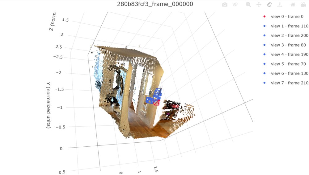
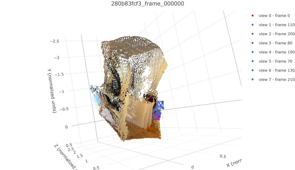
More funky geometry here (e.g. the predicted ceiling is curved instead of flat).
Scene 3, view 1 (GT top/predicted bottom):
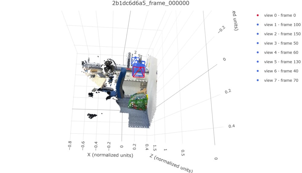
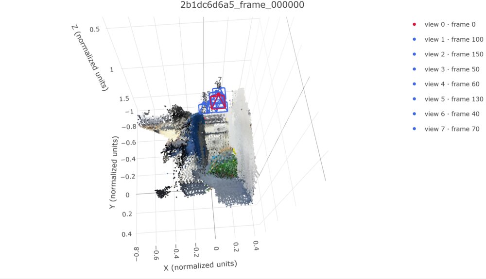
From a camera-aligned angle, our geometry doesn't look too bad.
Scene 3, view 2 (GT top/predicted bottom):
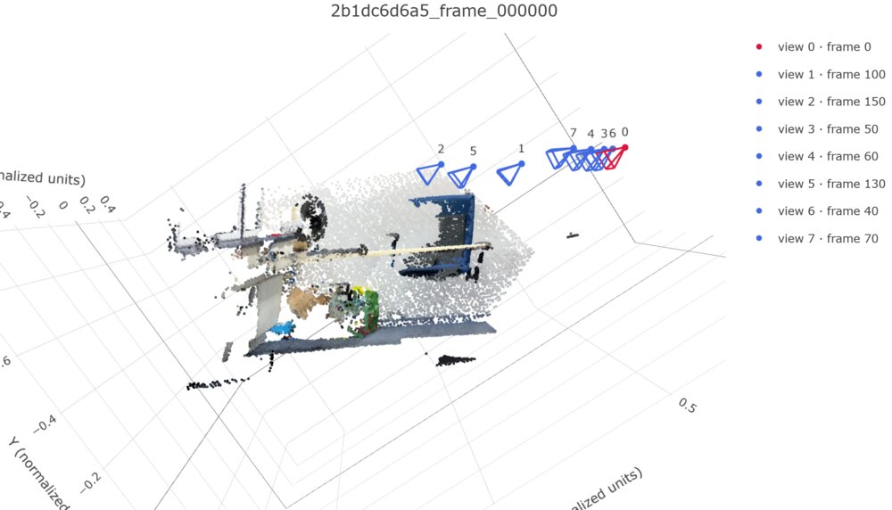
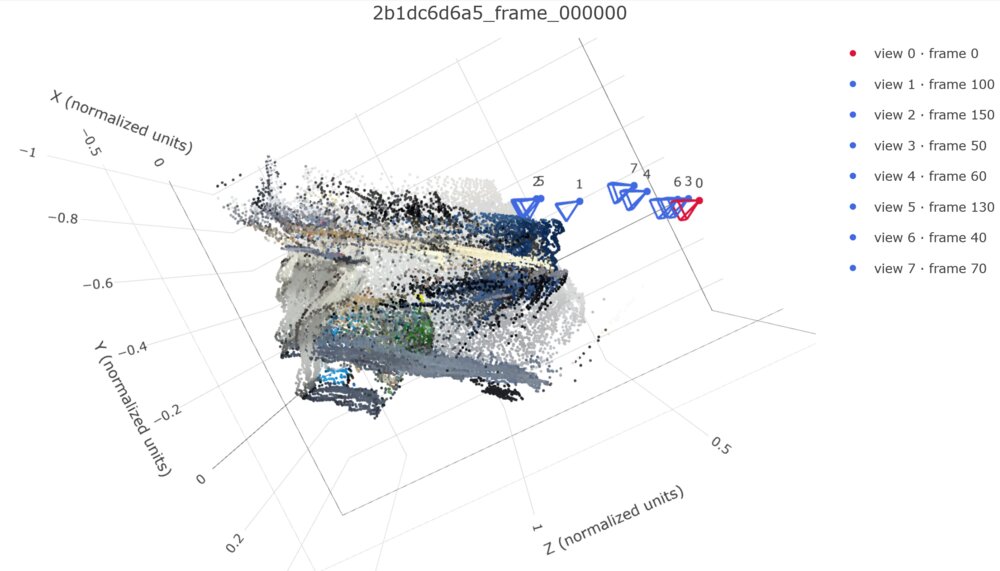
From a camera-unaligned angle, our geometry looks pretty bad, with the chair once again smearing/scattering in the direction of the viewing axes.
Discussion
In general, across the different scenes, we see a pattern where the geometry looks somewhere between okay and bad from viewing angles that are closer to the original camera angles, then looks very bad from angles not aligned with the original viewing angle. The biggest trend with geometry errors is that objects appear to be somewhat stretched/smeared, typically in a direction roughly parallel to the viewing axes, and the points are typically scattering away from the cameras rather than towards them. We do also see a few genuine hallucinations in the predictions, such as the copied bookshelves in scene 0 and the phantom half door in scene 2.
3.3. Bonus: Analysis and Exploration
For this section, I implemented an additional point prediction head in addition to the camera and depth heads from Q3.2, both to see the performance of a point head and to see if adding a point head would affect the predictions of the existing camera and depth heads. For the architecture, I used a very similar architecture to the depth head from Q3.2, with a few changes: I bumped up the # of output channels from 1 to 3, removed the confidence output, and changed the output of the final layer from $exp(x)$ to $sign(x)\cdot exp(x)$ (where $x$ is the output of the previous layer) in order to allow for negative coordinates in the output. The loss used was L1 between the GT and predicted points, masked by depth validity, with a point loss weight of 1 (compared to the default weights of 5 and 1 for the camera and depth losses, respectively).
Loss Curves
All training settings were kept the same as in Q3.2.

Visualizations
Scene 0, view 1 (GT top/depth head middle/point head bottom)
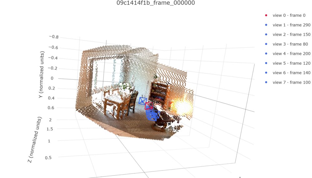
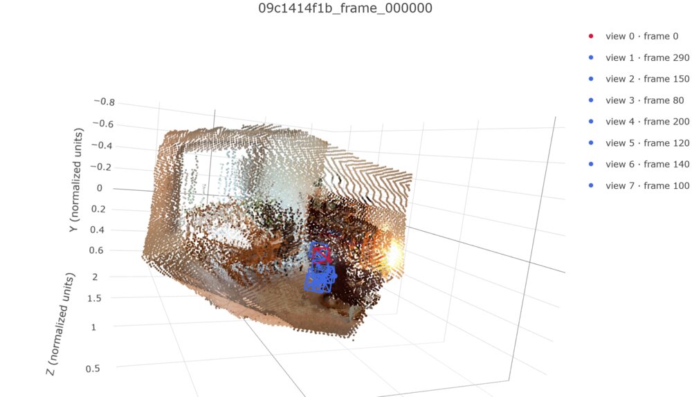
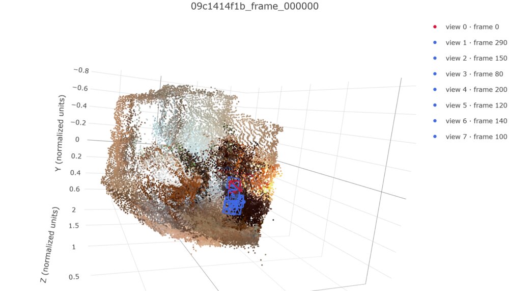
Here, the depth prediction appears somewhat improved relative to our prediction in Q3.2, although it's still noticeably fuzzier than + distorted relative to the GT, plus there still appear to be two bookshelves. Comparing the depth and point head predictions, we see that the depth head prediction appears significantly crisper and has more distinguished features than the point head prediction, but that the point head may have predicted a slightly smaller table (closer to the GT) compared to the depth head.
Scene 0, view 2 (GT top/depth head middle/point head bottom)
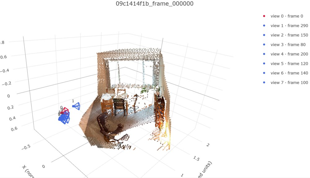
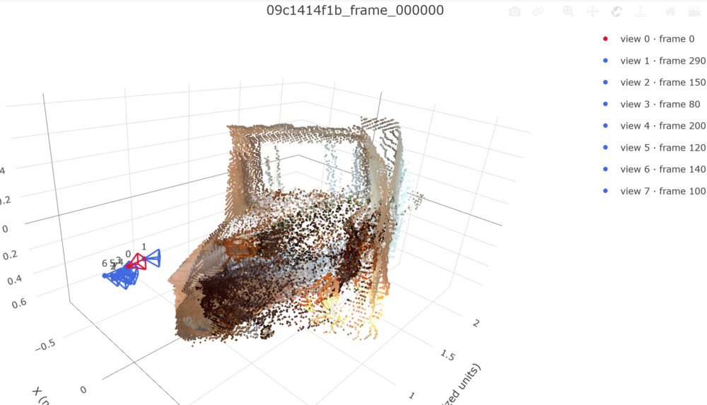
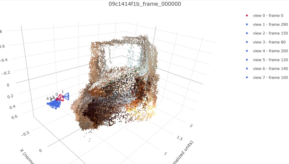
Looking at the same scene from another angle, we see that the geometry of the two predicted point clouds still appears "smeared" or scattered compared to the GT. Comparing the depth and point head predictions again, we see that although both look pretty bad, the depth head prediction appears to have more definition on the middle-left dining chair and the back of the bottom-left armchair than the point head.
Scene 2, view 1 (GT top/depth head middle/point head bottom)
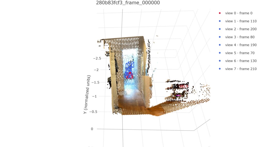
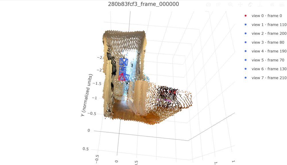
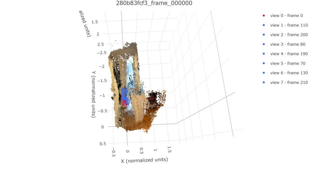
Taking a look at another scene, we actually see a pretty big difference between the depth and point head predictions -- the point head predicts the door closer to the wall (correct) and the shoe rack closer to the door (incorrect), whereas the depth head predicts a half-door that is partially open (very incorrect) and the shoe rack further from the door (correct). Neither gets either the door or the shoe rack completely correct, but we do get to see here that the predictions of the two heads need not be consistent with each other (as they are independent heads).
Q2.3 Comparison
Scene 0, view 1 (Q3.2 top, Q3.3 bottom)
Comparing the two models' predictions, we see that our new model has much nicer-looking tables and slightly less cloning on the bookshelf compared to our Q3.2 model, despite both models ostensibly having the same input-to-depth layers.
Scene 2, view 1 (Q3.2 top, Q3.3 bottom)
Although both models got the door and shoe rack in this scene wrong, we see that the Q3.3 model is much closer to being correct than the Q3.2 model. That is, the Q3.3 door is closer to being closed than Q3.2's, and the Q3.3 shoe rack is further away from the door than Q3.2's.
Metrics Comparison
val - No point loss |
val - With point loss |
test - No point loss |
test - With point loss |
|
|---|---|---|---|---|
| Depth AbsRel | 0.157 | 0.128 | 0.164 | 0.153 |
| Depth δ1 | 0.796 | 0.850 | 0.782 | 0.832 |
| Rotation AUC ($5^\circ$) | 0.173 | 0.204 | 0.174 | 0.210 |
| Rotation AUC ($15^\circ$) | 0.482 | 0.523 | 0.478 | 0.528 |
| Rotation AUC ($30^\circ$) | 0.679 | 0.704 | 0.687 | 0.717 |
| Translation AUC ($5^\circ$) | 0.014 | 0.021 | 0.006 | 0.016 |
| Translation AUC ($15^\circ$) | 0.084 | 0.093 | 0.053 | 0.082 |
| Translation AUC ($30^\circ$) | 0.195 | 0.202 | 0.167 | 0.203 |
| Joint Pose AUC ($5^\circ$) | 0.006 | 0.005 | 0.002 | 0.003 |
| Joint Pose AUC ($15^\circ$) | 0.072 | 0.068 | 0.032 | 0.055 |
| Joint Pose AUC ($30^\circ$) | 0.180 | 0.175 | 0.144 | 0.181 |
As far as metrics go, we can see a noticeable improvement across every metric going from the no-point-loss model to the with-point-loss model, across both val and test. The same goes for our visualizations, where the with-point-loss model has higher-quality and less-egregiously-geometrically-incorrect depth head predictions than the no-point-loss model. This signals that the addition of a point head, despite being independent of the camera and depth heads, has nonetheless improved the quality of our camera and depth heads' predictions.
Comparing the output of the depth and point heads, we see from the visualizations that the depth head's output appears to be significantly more well-defined in terms of visible features than the point head's, and the geometry is maybe a little cleaner; that said, we did also see a case where the point head had more correct geometry than did the depth head, indicating that the point head is interpreting its input features in a way that is meaningfully different from the depth head.