A. Neural Volume Rendering
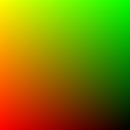
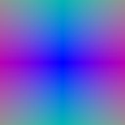
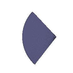
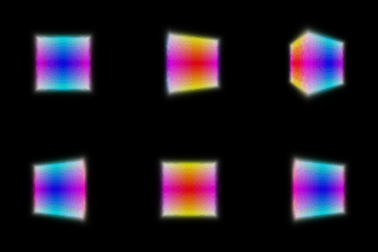
2. Optimizing a basic implicit volume
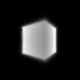
2.2. Loss and training
Output:
Box center: (0.25021326541900635, 0.2505703866481781, -0.000513455830514431)
Box side lengths: (2.0050556659698486, 1.5035252571105957, 1.5032978057861328)
Rounded:
- Box center: (0.25, 0.25, 0.00)
- Box side lengths: (2.00, 1.50, 1.50)
2.3. Visualization
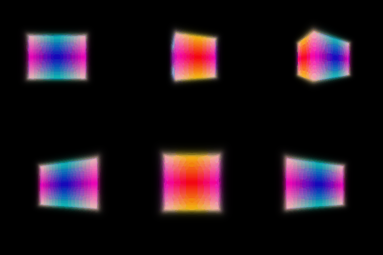
This GIF matches the one in the assignment README.
3. Optimizing a Neural Radiance Field
Network
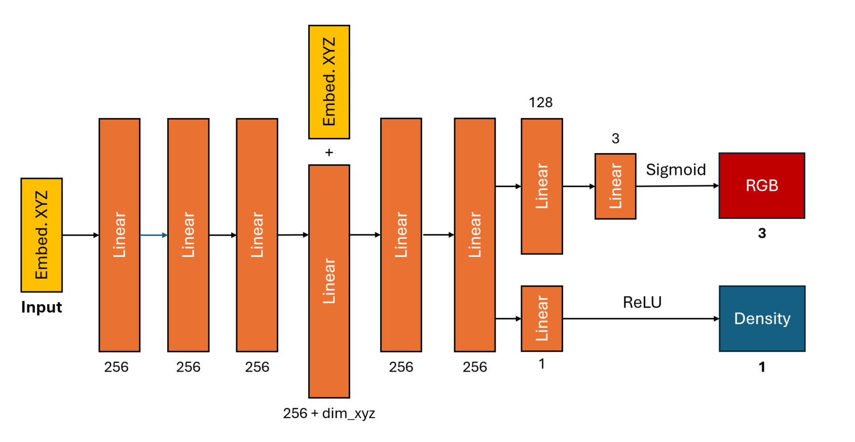
(+ represents concatenation.)
For the neural network, I used an architecture almost identical to the one used in the original NeRF paper (with minor modifications: less layers, no directional embedding, etc.). All transitions between layers utilized ReLU activation aside from the final linear layer into the RGB output, which used a sigmoid activation to map to the range $(0,1)$.
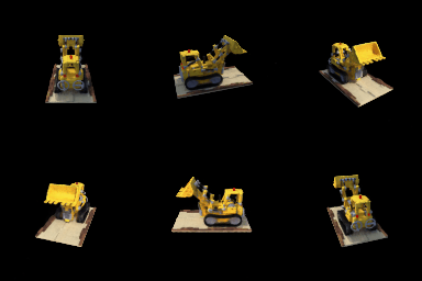
Output
4. NeRF Extras
4.1 View Dependence
Network
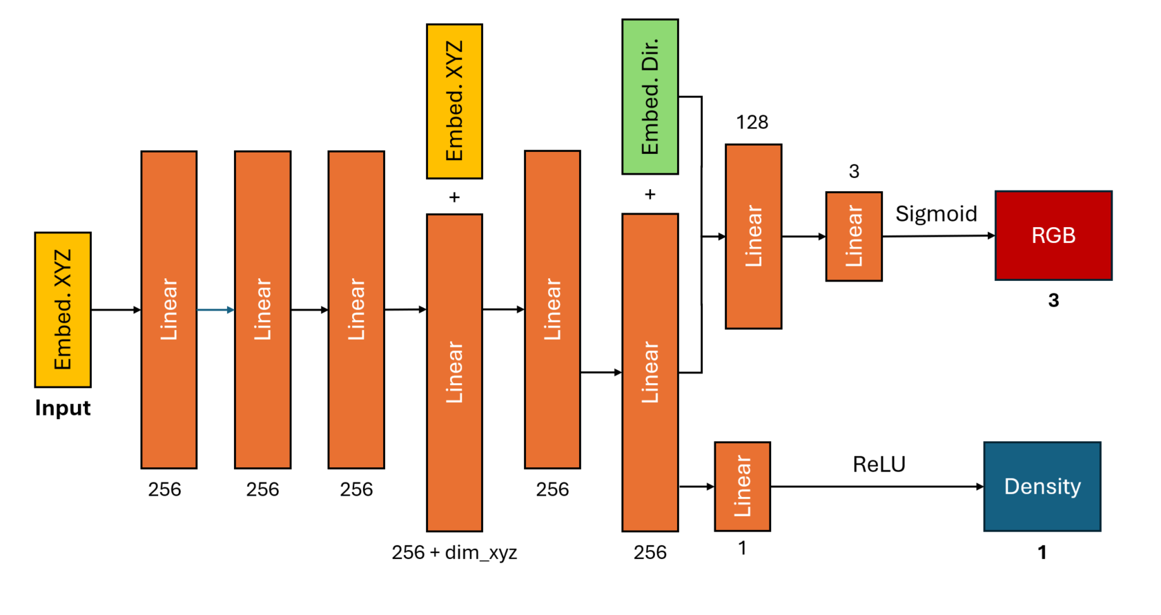
This architecture was almost identical to the one I used for Q3, with the exception of a concatenated direction embedding in the input layer to the final pre-RGB linear layer. Notably, the direction embedding was not passed to the pre-density linear layer, which received only the 256-vector from the preceding linear layer.
Output & Discussion
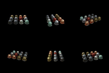
Increased view dependence allows the NeRF to better depict view-dependent aspects of an object's appearance - one notable example is specular reflections, which reflect light in a particular direction, and thus should only be visible from some views and not others. This can be seen in the balls in the GIF, where parts of the ball appear shinier from some angles than the same parts do from other angles.
One cost of view dependence is generalization - since the NeRF now takes an additional parameter (direction, or some function of direction), novel view directions not seen during training may not produce the desired results if the direction parameter acts unpredictably (or otherwise harms the render). In comparison, view-independent NeRFs should be more stable/generalize better, since a position + direction query that is out-of-distribution may still be in-distribution without the direction component, as said position may still have been visible from other views.
4.2 Coarse/Fine Sampling
Network
The same architecture as in Q3 was used for both my coarse and fine network, with both networks being trained jointly during the training process. For the input points to the fine network, I used the concatenation of the original coarse sample points and a "finer" weighted sample of ray points, as in the original NeRF paper. The fine network and concatenated coarse + fine sample points were used to generate all results.
Discussion
In most cases, we'd expect the quality of the coarse-fine (hierarchical) network's renders to be higher. Compared to our basic NeRF, which sampled uniformly across every ray, the coarse-fine approach uses uniform sampling only for the coarse points, then uses a weighted sampling for the fine sample points. The weights generally are higher for regions that are predicted to be part of an object/higher density, therefore the fine sample points will be be more heavily clustered around parts of an object. Even with the same # of overall sample points, this can result in better-resolution renders of objects, since the rays will feature less queries of blank space (which don't contribute much to the render) and more queries around objects (which can help better capture granular detail, notably surface details).
The trade-off is that the coarse-fine network will be much slower. Notably, the coarse-fine network involves training two networks independently (the coarse network and the fine network), which (roughly) doubles the amount of work overall in terms of network training. The coarse-fine network also requires two different sets of network queries (one to the coarse network, then one to the fine network), where querying the fine network for a pixel $(u,v)$ requires first obtaining the coarse network predictions for that same network, preventing easy parallelization and thus resulting in a slower inference speed. Finally, the coarse-fine network makes more queries for the same # of query points (on the fine network) than the base network based on the original NeRF paper -- the original NeRF paper takes the set of fine sample points as the concatenation of the original set of coarse sample points plus a newly sampled set, hence a rendering of $N$ fine points per ray actually requires querying a total of $M+N$ points per ray (where $M$ is the number of coarse sample points per ray, $M<N$).
Results

4.3 VolSDF
Discussion
In the equation itself, $\alpha$ is just a scalar multiplier on the output density. Practically speaking, $\alpha$ can be seen as the "true" density of a fully occupied opaque object, as the terms multipled by $\alpha$ are $\in(0,1)$, hence $\alpha$ is the least upper bound on density.
$\beta$ can be interpreted as modifying how "hard" or "soft" object boundaries are in the output density. In the equation, the density for large values of the SDF (far away from all objects) is approximately 0, the density at an object boundary (SDF = 0) is $0.5\alpha$, and the density for very negative values of the SDF (far inside an object) is approximately $\alpha$. $\beta$ controls the transition between these values around an object boundary, with larger values of $\beta$ causing a slower transition.
- How does high beta bias your learned SDF? What about low beta?: High $\beta$ biases the learned SDF toward a smoother/blurrier surface, as higher values of $\beta$ penalize small errors in the learned surface less strongly/more weakly and thus allow the learned SDF to "get away" with a less exact surface (see part 3 for more explanation). In contrast, lower $\beta$ biases the learned SDF toward learning a sharper surface, as lower values of $\beta$ result in larger penalties on misclassified regions. However, there is no systematic bias in that changing the value of $\beta$ will not consistently cause the surface to shift inward or outward.
- Would an SDF be easier to train with volume rendering and low beta or high beta? Why?: An SDF would be easier to train with higher $\beta$ (i.e. more smoothing). The reason is that the loss (L1/L2 on pixel values) only directly depends on the SDF in that the density values used for rendering are dependent on the SDF, hence all gradients have to flow through the SDF$\to$density transformation function to reach the SDF. Said transformation has very small gradients when the input to the exponential term is large in magnitude (since said input is always negative), which impede training. Higher values of $\beta$ decrease the magnitude of the input to the exponential, which increases the region of significant gradients and thus helps training.
- Would you be more likely to learn an accurate surface with high beta or low beta? Why?: You would be more likely to learn an accurate surface with low $\beta$. As $\beta\to0$, the density function approaches $\rho(s)=\alpha I_{s\leq0}$, i.e. $\alpha$ when the SDF is $\leq0$ and 0 otherwise, i.e. the dropoff in density inside/outside is sharper. Another interpretation is that lower values of $\beta$ push the density towards either 0 or $\alpha$ - under this interpretation, any misclassified regions will have their density be off by a larger value (as the lower $\beta$ pushes the density toward the wrong extreme), increasing the penalty and thus encouraging the SDF to learn a better surface. In contrast, with higher $\beta$, since the density transition is smoother, there is a smaller penalty for getting the surface slightly wrong, hence the surface is likely to be less accurate.
Network
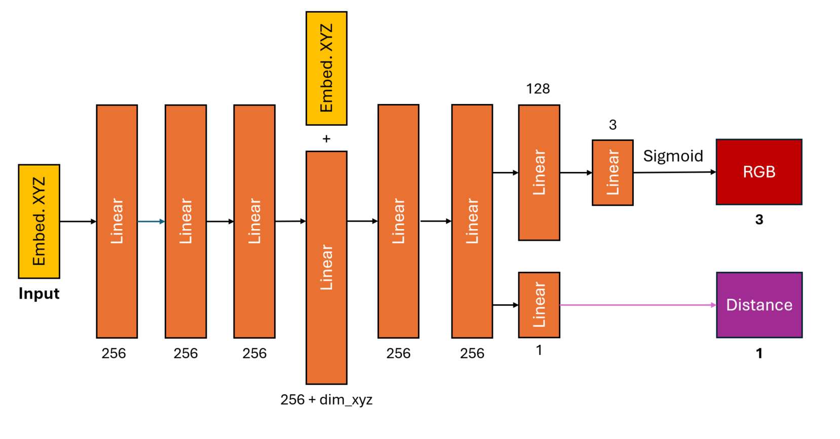
This architecture was almost identical to the one I used for Q3, with the exception of my replacing the previous density head with a (near-identical) distance head. Notably, the distance head does not include an activation function between its final linear layer and the distance output, i.e. the distance output is simply the raw output. (This is due to the distance representing the value of an SDF, which is theoretically unbounded in both the negative and positive directions.)
Results
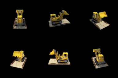
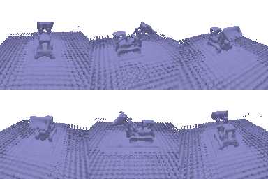
Parameters (default): $\alpha=10.0,\;\beta=0.05$
As mentioned, I simply used the default parameters, and since the output rendered GIF looked decent enough (as far as I could tell, given the limited resolution), I didn't feel the need to try and optimize the parameters. That said, my output geometry does have a lot of bad geometry around the base of the object - I ignored these, since they didn't show up in the final rendering (were predicted to have 0 density, perhaps), but if I wanted to try and limit the geometry to only the "true" objects (as in the assignment's geometry GIF), I might speculate that the network is having trouble learning the SDF and therefore increase $\beta$ in order to try and help the network train better, as I mentioned in part 2 above.
B. 3D Gaussian Splatting
5. 3D Gaussian Rasterization
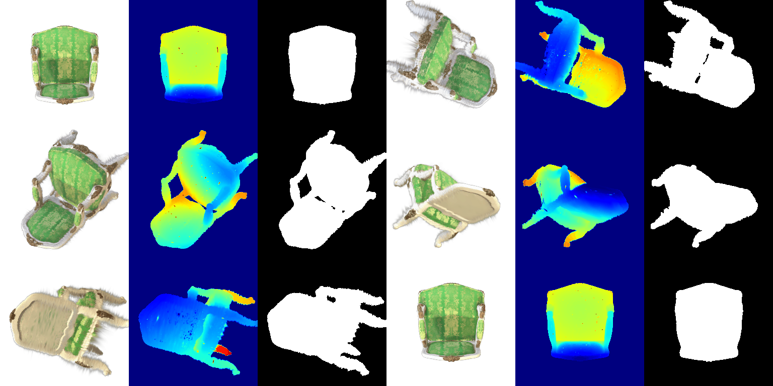
6 Training 3D Gaussian Representations
Parameters:
- # iterations: 1000
- Learning rates:
- Opacity: 0.05
- Scales: 0.005
- Colors: 0.005
- Means: 0.0005
Output:
[*] Evaluation --- Mean PSNR: 30.082
[*] Evaluation --- Mean SSIM: 0.945
7 Extensions
7.1 Rendering Using Spherical Harmonics
GIFs
Original, Q5.5:
With spherical harmonics:
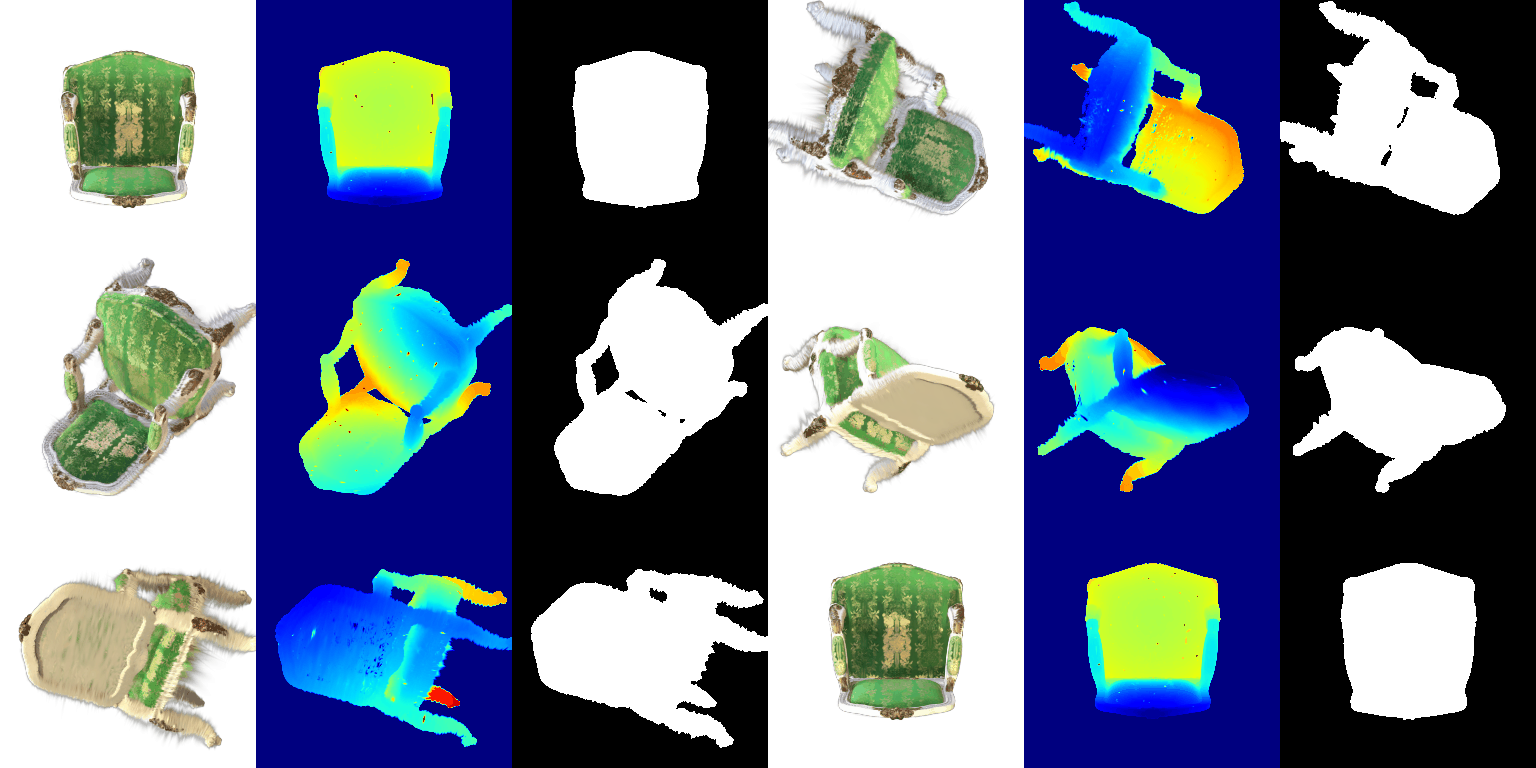
Comparisons
(Top is the base/original from Q5.5, bottom is with spherical harmonics [SH])
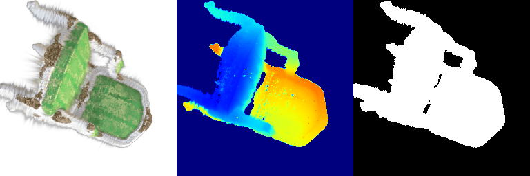

The main difference visible is the color of the green parts of the seat - where the original had a fairly light green all around, with some slightly darker regions on the seat back, the SH render has significantly darker green on the chair back and front (the faces facing the camera), but retains the same light green on the chair cushion (facing slightly away from the camera). The SH render also has slightly darker brown on the brown parts of the chair.
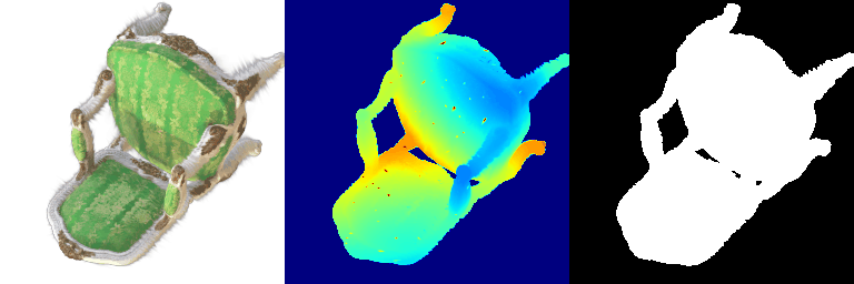

Similar to previous, the SH render has much more pronounced dark regions on the chair back and front. Compared to the base render, the shadow (if it is a shadow) on the seat cushion is much less sharp, and the rest of the seat cushion is darker than in the base render. Most notably, where the green regions on the base version seem fairly flat (i.e. the green is constant across the entire region), the SH render has much more complex coloration across the board. (This can also be seen in the white and brown regions of the chair, which appear somewhat more detailed in the SH render).
One noticeable detail here is that in the second SH render, the entire seat cushion appears to be (to some extent) in shadow, whereas the same is not true in the first and third SH renders.
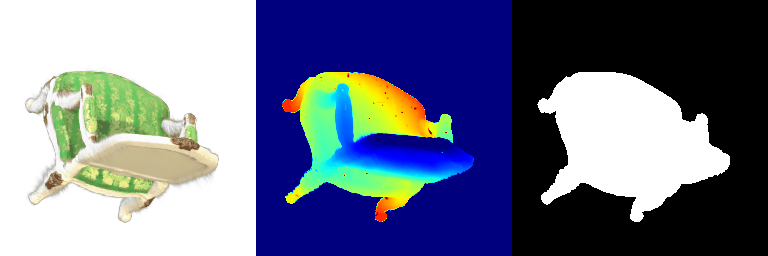

Similar to previous, there is more contrast between the different shades of green in the SH render vs. the base render (the SH render has brighter highlights, darker shadows, and richer greens overall). Consequently, the yellow patterning on the top of the seat cushion are somewhat difficult to see in the SH render compared to the base render due to the brighter green - this may be due to some kind of reflection/glossiness on the original chair. The brown regions of the chair also appear darker in the SH render.
Overall, the biggest difference between the base and SH renders is in how the appearance of the green cushions varies based on viewing angle. In the base render, all parts of the green cushions are essentially the same color from every angle. In contrast, in the SH renders, different parts of the chair appear brighter or darker from different angles (e.g. the top part of the chair cushion is very bright in the third render, fairly bright in the first, and somewhat dark in the second). Beyond this, the coloration of the SH renders generally just appears richer, more complex, and more varied overall, whereas the base renders appear somewhat flat/lacking in color variation in comparison.
7.2 Training On a Harder Scene
Parameters:
- # iterations: 1000 (unchanged)
- Learning rates:
- Opacity: 0.05 (unchanged)
- Scales: 0.005 (unchanged)
- Colors: 0.005 (unchanged)
- Means: 0.02 -> 0.0002 (exponential decay)
Changes made:
- I implemented SSIM loss to try and boost performance. The SSIM loss was computed on 7x7 patches & averaged across the whole image, with the final loss being a weighted sum of MSE (0.8x) and SSIM loss (0.2x).
- Rather than using a fixed learning rate of 0.0005 for the Gaussian means, I used a simple scheduler that initialized the learning rate at 0.02 and decayed exponentially to 0.0002 over the course of the 1,000 iterations.
- I switched from isotropic to anisotropic Gaussians.
Results
Baseline (Q6.2):
[*] Evaluation --- Mean PSNR: 17.685
[*] Evaluation --- Mean SSIM: 0.677
V2:
[*] Evaluation --- Mean PSNR: 18.507
[*] Evaluation --- Mean SSIM: 0.686
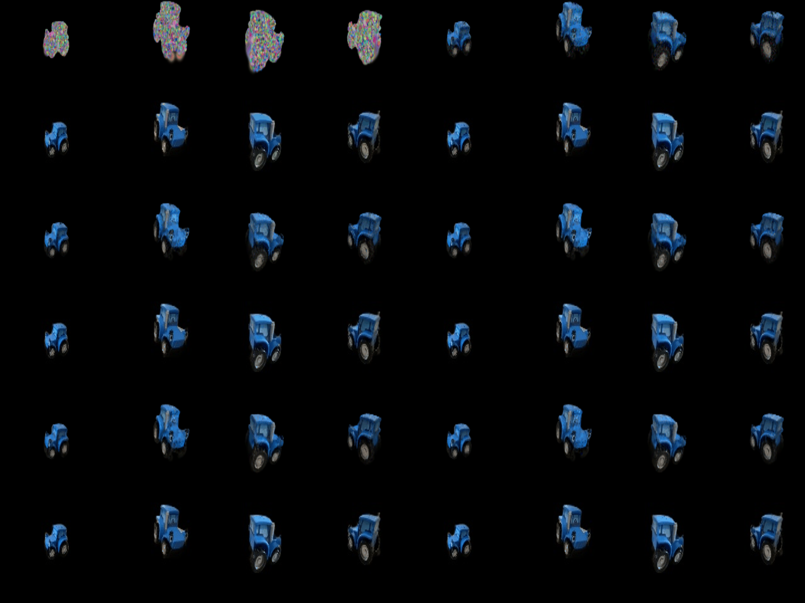
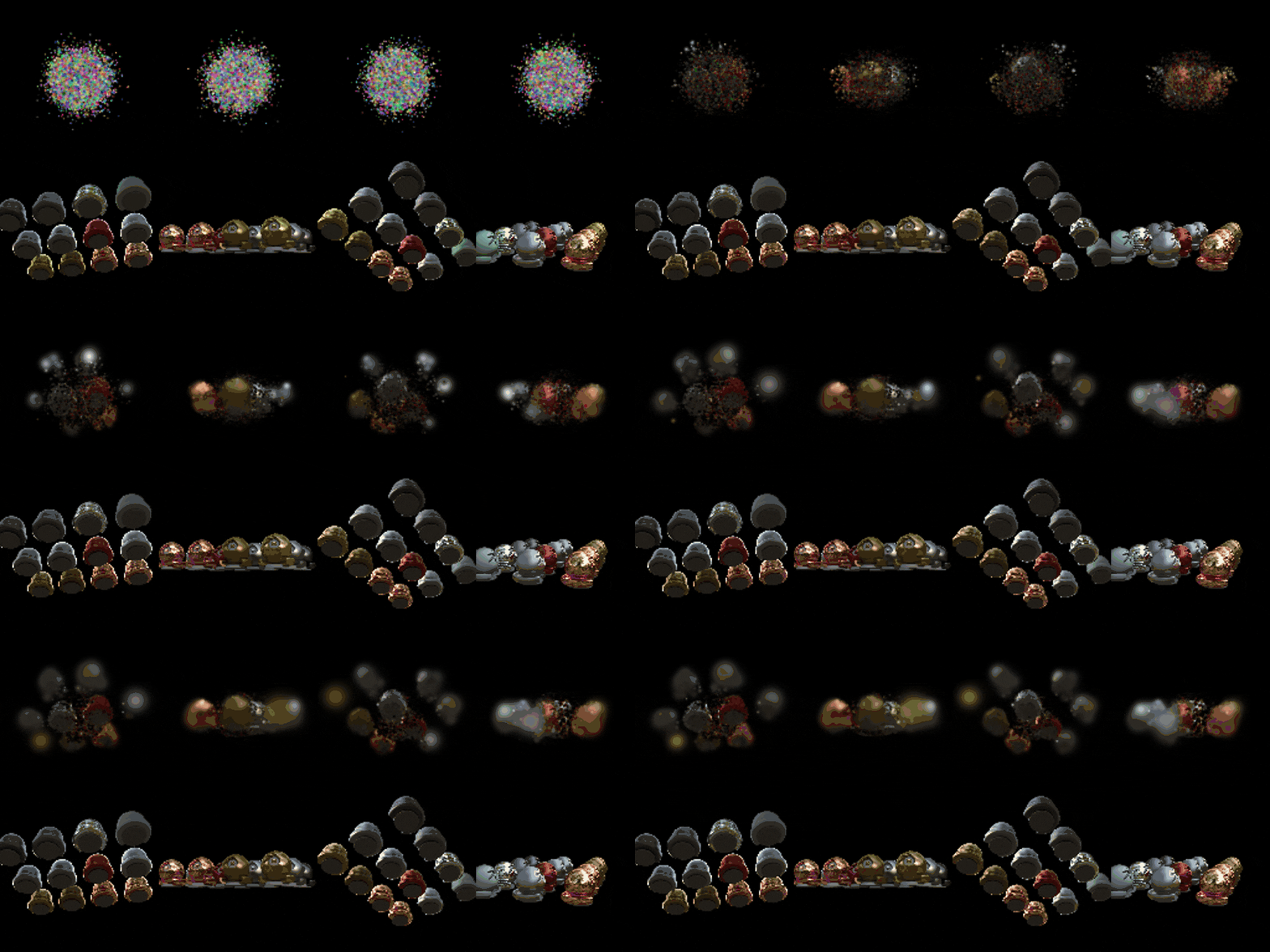
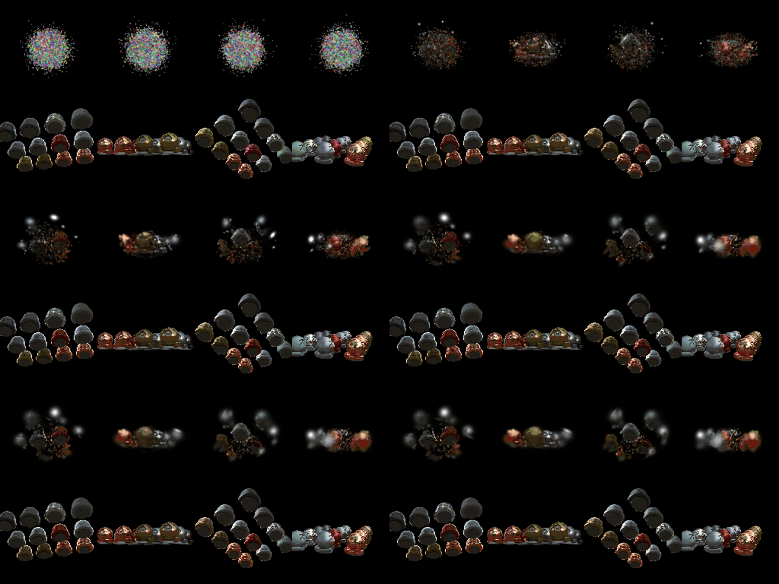
The improvement was very underwhelming to me; I think more iterations, a change to the Gaussian initialization strategy, and/or a different scheduling strategy with a higher Gaussian mean learning rate for the initial iterations may have helped, as it appeared (from the GIFs) that while the central objects had been learned relatively well, the Gaussians for the outside objects had not yet fully converged.
Progress GIFs
Baseline (Q6.2):
V2:
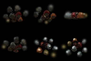
Final renders (base, then V2)
Baseline (Q6.2):
V2:
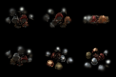
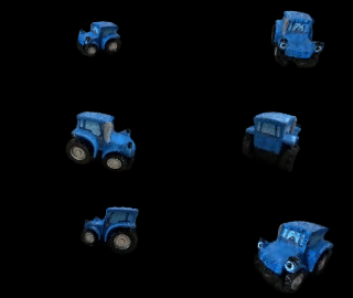
Unfortunately, it's hard to tell much of a difference between the various GIF pairs, and they all end up looking pretty bad in the final output. One thing I did notice is that it appears (based on the top row) that the Q6.2 baseline Gaussians spread out much faster and reached the correct positions much faster than my V2 Gaussians, but that those V2 Gaussians around the center objects (i.e. that were correctly positioned) were able to stabilize and obtain a sharper appearance faster than the Q6.2 baseline, which was both slower and had a blurrier final result. If I were to do this again (which I don't have time to, unfortunately :( ), I might (a) try to spread out the initialization of the Gaussians, either with a different initialization method or just by bumping up the randomness, and (b) have a less aggressive falloff on the learning rate of the Gaussian means in order to try and encourage them to spread out more in the early epochs before stabilizing and being refined in the later epochs.