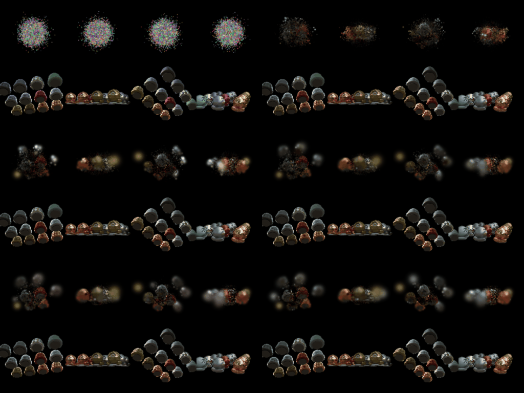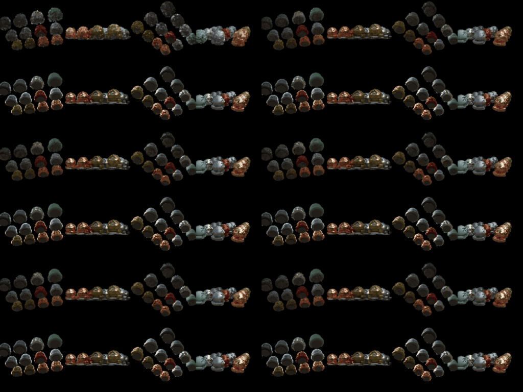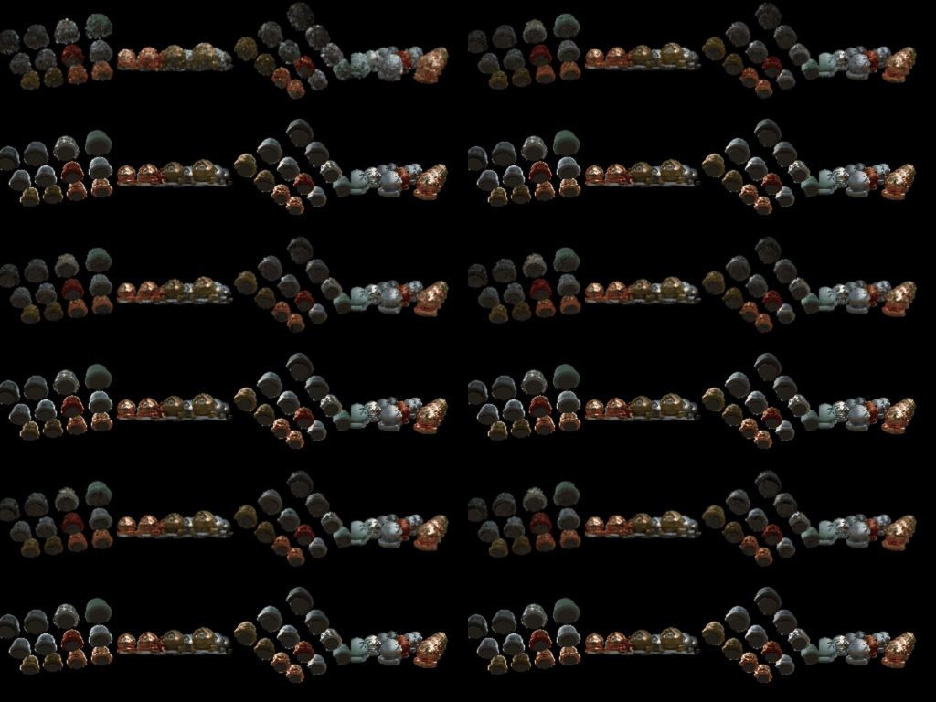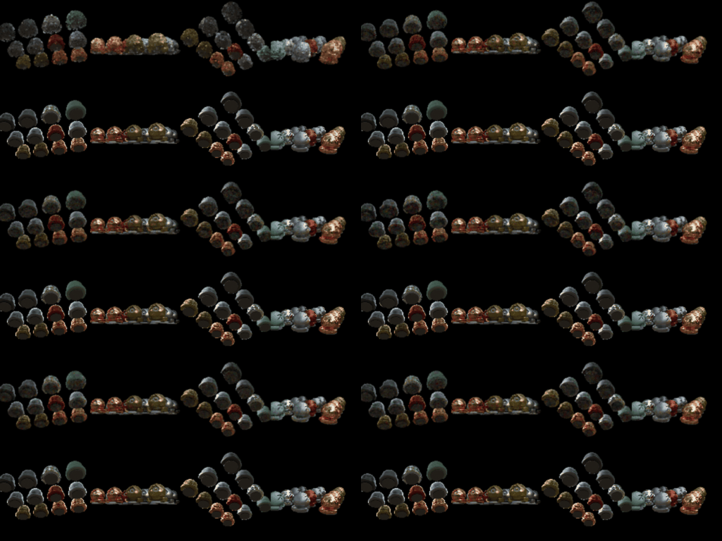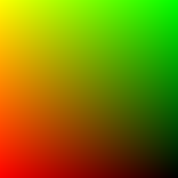
xy_grid)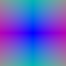
xy_grid)
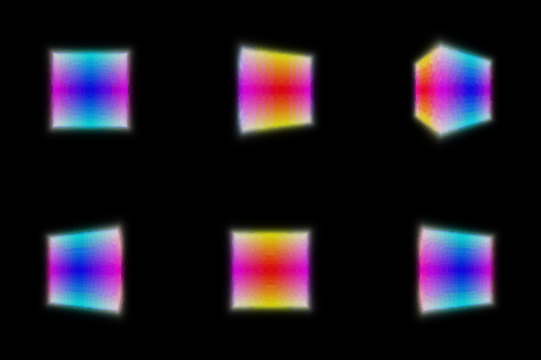
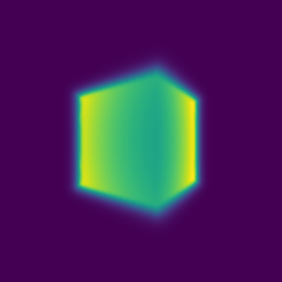
| x | y | z | |
|---|---|---|---|
| Box center | 0.25 | 0.25 | 0.00 |
| Box side lengths | 2.01 | 1.50 | 1.50 |
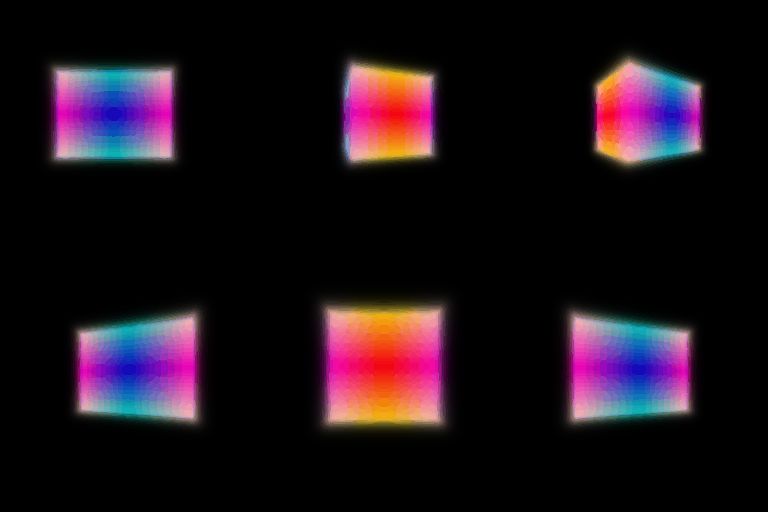
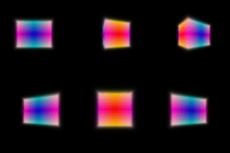
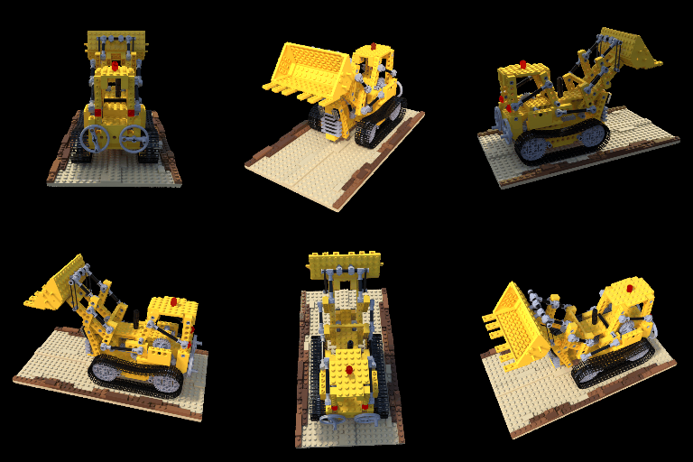
Final training loss (MSE, last epoch): 0.002985
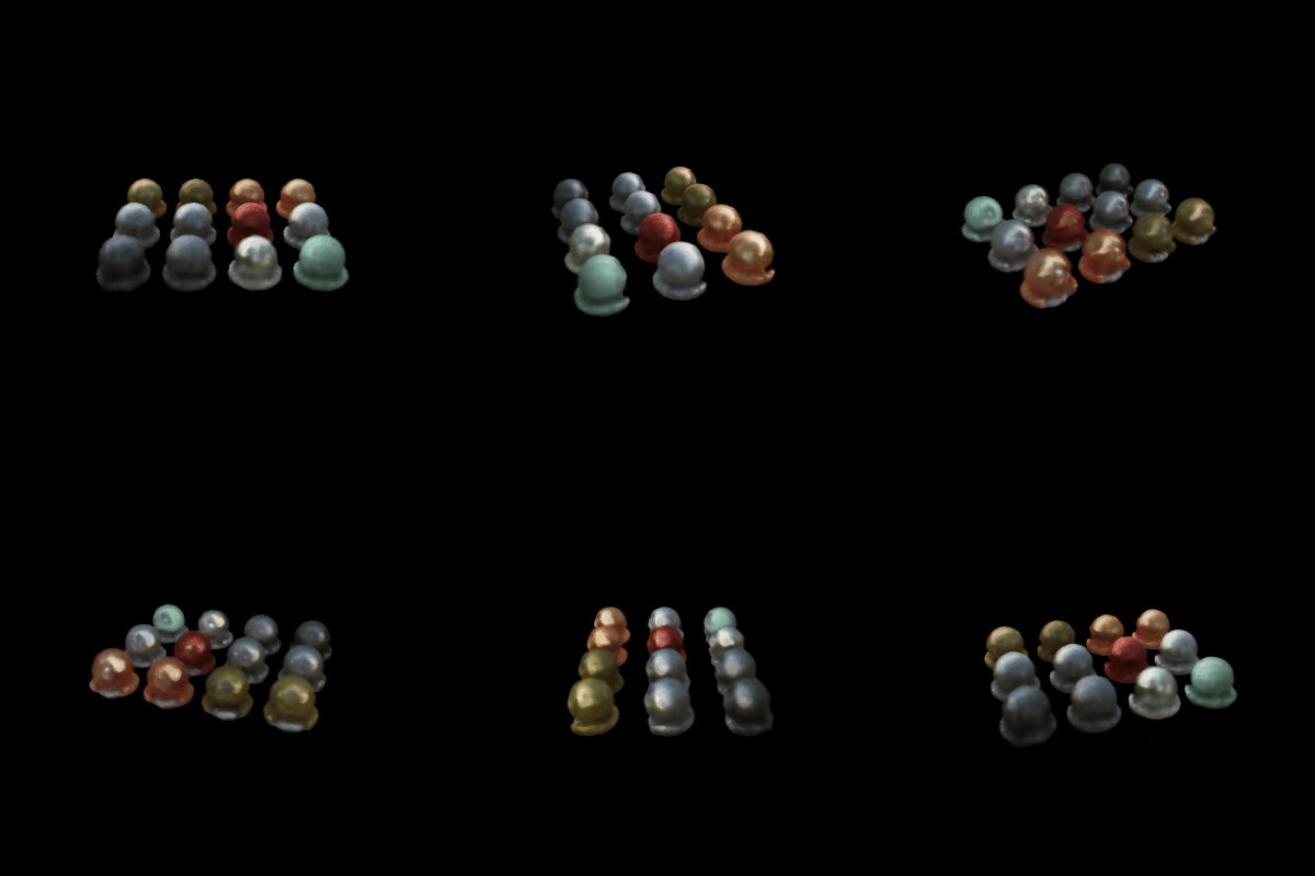
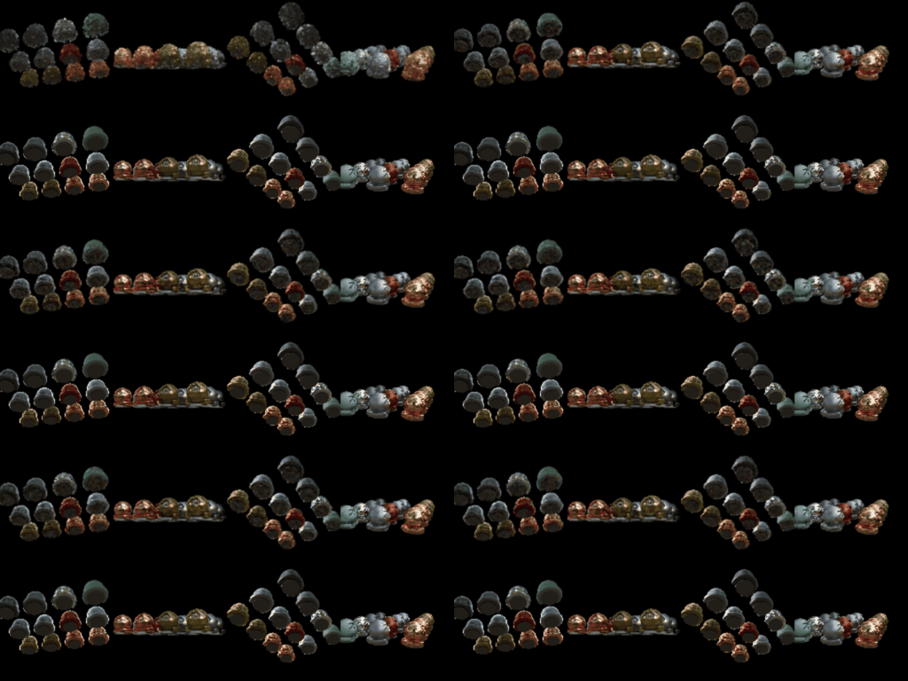
nerf_materials_highres)

| Materials, 128×128 | Mean PSNR | Mean SSIM | Parameters | Training speed | Training time (250 epochs) | Inference (128×128 frame) |
|---|---|---|---|---|---|---|
| Without view dependence | 23.625 | 0.870 | 481,796 | 21.3 it/s | 19.6 min | 233 ms (4.3 fps) |
| With view dependence | 24.308 | 0.884 | 582,020 | 18.6 it/s | 22.4 min | 266 ms (3.8 fps) |
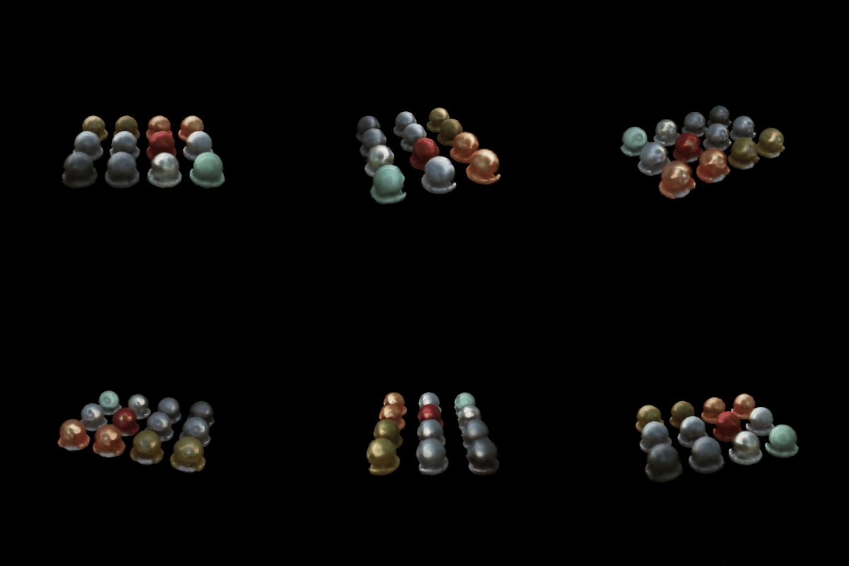
We see a clear improvement from using view dependence, both in the metrics and visually. It is most visible on the grey balls in the center, which for me showed the view dependence best. The scene is still fairly low resolution for major differences to show up. I think that with training at a higher resolution, we would have seen a larger gap in both the metrics and the visual quality.
The cost of view dependence is about 100K extra parameters for the direction branch and about 14% slower training and rendering (18.6 vs 21.3 it/s, 266 vs 233 ms per frame). The risk for generalization is that the network can explain the training views with view-dependent colour instead of learning the actual geometry, which would hurt novel views.
| Run | Mean PSNR | Mean SSIM | Parameters | Network evaluations per ray | Training speed | Training time (250 epochs) | Inference (per frame) |
|---|---|---|---|---|---|---|---|
| Lego 128×128, single network | 25.307 | 0.912 | 481,796 | 128 | 29.5 it/s | 14.1 min | 163 ms |
| Lego 128×128, coarse + fine | 25.712 | 0.921 | 963,592 | 128 + 256 = 384 | 11.0 it/s | 38.0 min | 507 ms |
| Materials 400×400 + view dependence, single network | 24.405 | 0.853 | 582,020 | 128 | 20.0 it/s | 20.9 min | 2.72 s |
| Materials 400×400 + view dependence, coarse + fine | 24.416 | 0.852 | 1,164,040 | 128 + 256 = 384 | 7.6 it/s | 55.0 min | 11.70 s |
The fine network evaluates the 128 stratified samples plus 128 importance samples drawn from the coarse weights. Each ray therefore costs about 3× the network evaluations of the single-network model, which matches the 2.6–2.7× slower training we measured. Rendering runs both passes as well, so inference is 3.1× slower on lego and 4.3× slower on materials at 400×400.
So we did not get any huge gain in quality overall (+0.4 dB PSNR on lego, essentially none on materials), but the runtime went up a lot, so for these scenes coarse/fine sampling does not seem worth it.
N/A
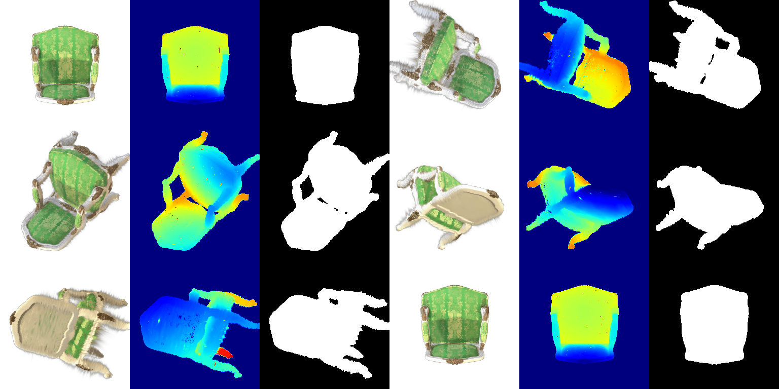
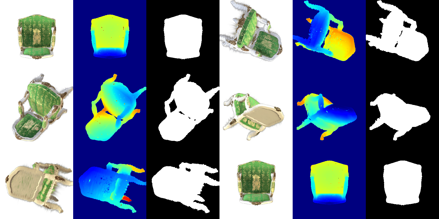
render.py (RGB, depth, mask)| Parameter | Learning rate |
|---|---|
| Opacities | 0.05 |
| Scales | 0.005 |
| Colours | 0.02 |
| Means | 0.0005 |
| Iterations | Mean PSNR | Mean SSIM |
|---|---|---|
| 1000 | 29.584 | 0.938 |
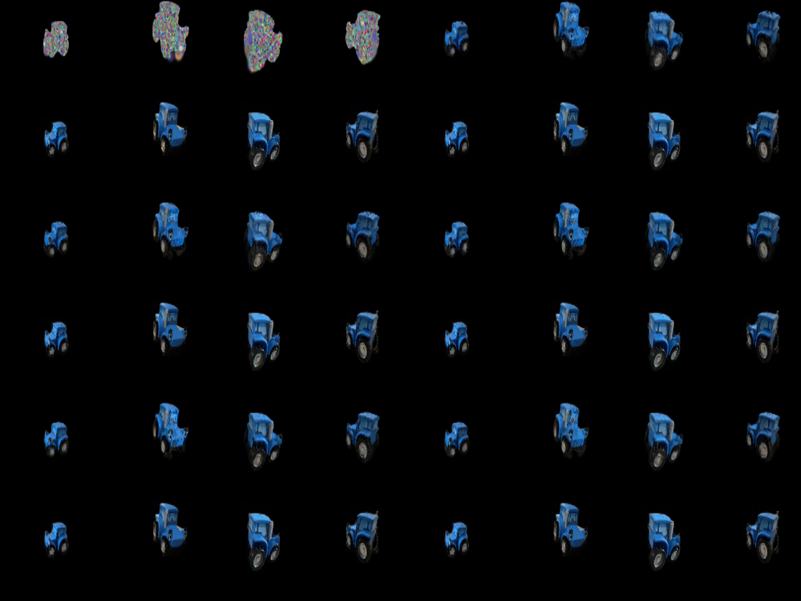
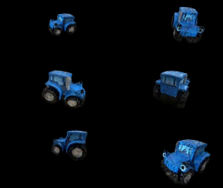
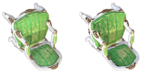
With spherical harmonics there is a bit more contrast on the objects and the details look much better. The back of the chair has a difference in colour with SH, whereas without it we don't see that difference. It also looks sharper than the render without SH.
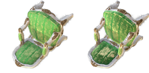
Same as frame 3: the back of the chair shows the difference in colour with SH that is missing without it, and it looks sharper with SH.
The Gaussian means are initialized from a point cloud predicted by MapAnything instead of the random init. The pipeline (GS/mapanything_init.py) has five steps:
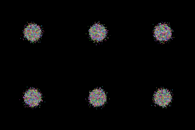
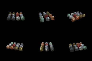
Each run adds one change on top of the previous one. All runs use 10,000 Gaussians, 1000 iterations at 128×128, and the Q6.2 learning rates: opacities 0.05, scales 0.005, colours 0.02, means 0.0005. Quaternions use 0.001 and higher-order spherical harmonics 0.0035 where they are trained.
| Run | Init | Gaussians | Colour | Loss | Mean PSNR | Mean SSIM |
|---|---|---|---|---|---|---|
| Baseline (Q6.2 setup) | random | isotropic | RGB | L1 | 18.456 | 0.683 |
| MapAnything init | MapAnything points + colours | isotropic | RGB | L1 | 23.431 | 0.868 |
| + anisotropic | MapAnything points + colours | anisotropic | RGB | L1 | 23.600 | 0.871 |
| + view dependence | MapAnything points + colours | anisotropic | SH degree 3 | L1 | 25.211 | 0.901 |
| + SSIM loss (best) | MapAnything points + colours | anisotropic | SH degree 3 | 0.8 L1 + 0.2 (1 − SSIM) | 25.349 | 0.910 |


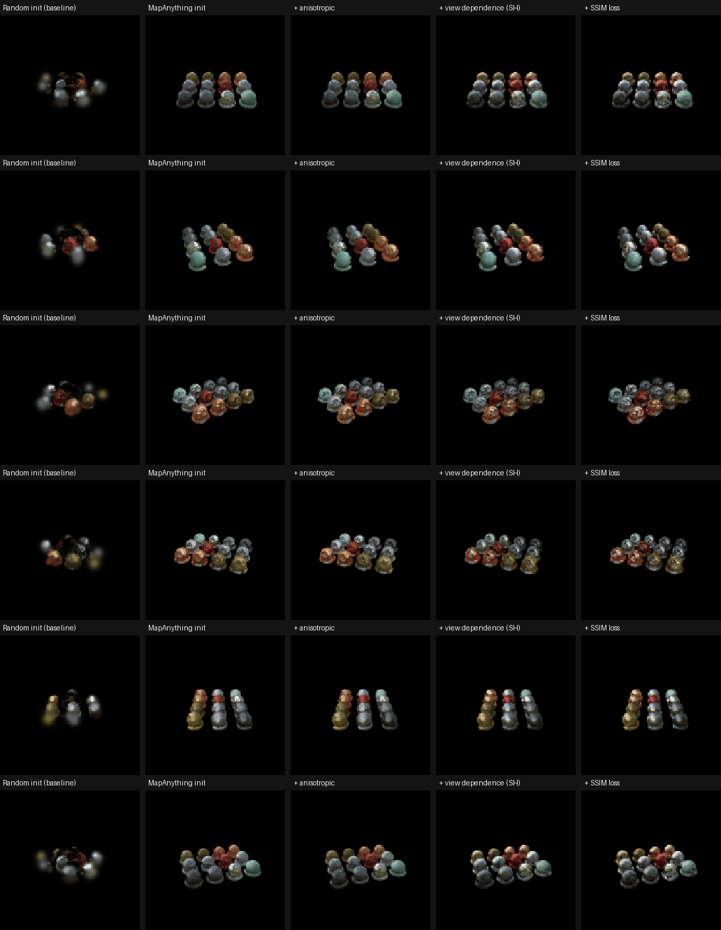
The highest gain came from using an external model (MapAnything) for the initialization: PSNR went from 18.456 to 23.431 and SSIM from 0.683 to 0.868, and the loss plateaued a lot earlier. Initializing from this model is easier than starting from a random init and saves training time. With the random init our scene did not even converge in the given iterations.
Anisotropic Gaussians gave a small gain (23.431 to 23.600 PSNR, 0.868 to 0.871 SSIM), since each Gaussian can stretch along the surface instead of being a sphere. View dependence gave the second largest gain (23.600 to 25.211 PSNR, 0.871 to 0.901 SSIM), since the materials are shiny and their colour changes with the viewing direction, which a single RGB colour per Gaussian cannot represent.
Adding the SSIM loss also helped (25.211 to 25.349 PSNR, 0.901 to 0.910 SSIM), but by a smaller margin than the init and view dependence. It is about the same as anisotropic in PSNR, and larger in SSIM since that is the metric it directly optimizes.