Sphere init, with smoothness lossSphere init, no smoothness loss
Bounding-box sphere initCow init, with smoothness loss
The smoothness loss gives far fewer spikes, even from a worse initialization such as a larger sphere. Even with it, the gaps between the chair legs are not modelled well. An initialization closer in scale to the target (the bounding-box sphere) gives a better result. For fun, I also tried starting from the cow mesh to see what it would give.
2. Reconstructing 3D from single view
2.1 Image to voxel grid
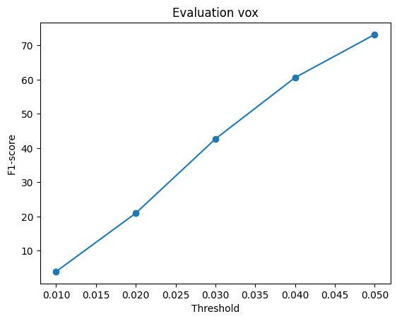
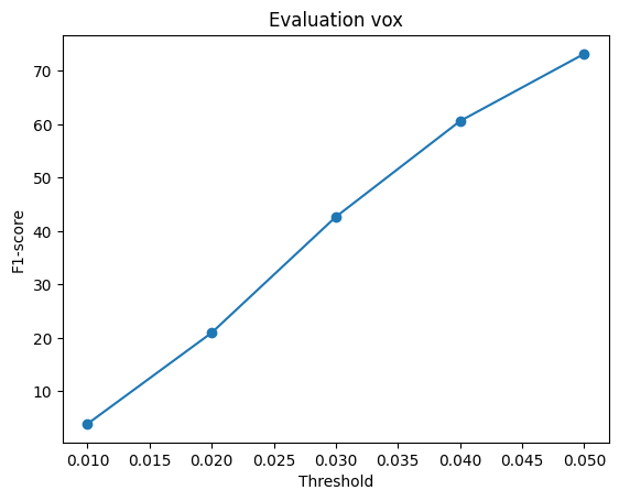
F1@0.05: 73.19
Test example 0Test example 400Test example 250
F1 vs. threshold
2.2 Image to point cloud
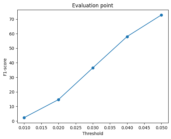
F1@0.05: 72.86
Test example 150Test example 450Test example 550
F1 vs. threshold
2.3 Image to mesh
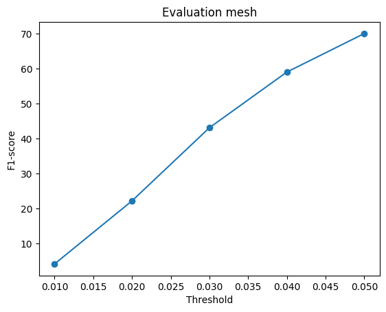
F1@0.05: 70.02
Test example 0Test example 500Test example 150
F1 vs. threshold
Comparison
Representation
F1@0.05
Voxel grid
73.19
Point cloud
72.86
Mesh
70.02
Voxels: visually, I found the voxel predictions the best of the three. They could be made more fine-grained by predicting at a higher voxel resolution, but the cost grows cubically with resolution, so beyond a point this becomes computationally inefficient.
Mesh: the predicted meshes are still very spiky. Deforming a sphere into a chair is hard; an initial mesh that is a better fit to the chair shape would likely help.
Point cloud: even though its F1 is close to the voxel model's, the predictions do not look as good visually.
Common failure modes: all models struggle to capture fine details such as chair legs. They also do better on generic chairs than on less common ones such as sofa chairs, since generic chairs are far more abundant in the training set. At times the model simply outputs a standard chair rather than the one shown in the image.
Loss and F1 can be misleading: monitoring the loss and the evaluation metric did not always lead to better-looking results, especially for the point cloud and mesh models, which are compared using only 1000 sampled points. At that sampling density, spikes, stray points and missing thin parts barely change the score, so a visually worse prediction can score as well as a better one.
2.4 Effect of hyperparameter variations
Early in training, the voxel model frequently predicted completely empty grids. To counter this, I added a weight to the BCE loss for ground-truth voxels that are occupied (pos_weight 2). This led to faster convergence and fewer completely empty predictions. I then added a Dice loss term (w_dice 1) on top to see whether it would further improve the model's performance.
Voxel model loss
F1@0.05
BCE (pos_weight 2)
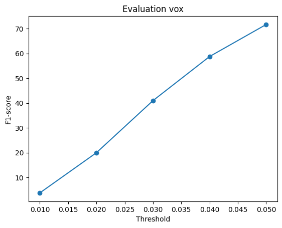
71.64
BCE (pos_weight 2) + Dice
73.19
Adding the Dice loss gave only a very small gain in F1, but the predictions themselves were slightly better and cleaner.
Test example 0, without DiceTest example 0, with DiceTest example 400, without DiceTest example 400, with DiceTest example 250, without DiceTest example 250, with DiceF1 vs. threshold, without DiceF1 vs. threshold, with Dice
2.5 Interpreting the model
Voxel confidence map. Each cube's size and color show the predicted occupancy probability: large and green is high, small and red is low. Voxels below 0.1 are not drawn. Both models use the same scales.
Test example 0Test example 200Test example 400
I found this visualization really cool, since it shows the model's uncertainty in 3D.
With Dice, the predictions are much more confident. BCE scores each voxel separately, while Dice scores the overlap of all voxels at once, which pushes each probability towards 0 or 1.
Higher confidence does not mean higher accuracy. The wrong voxels are also confident, so the Dice model is probably poorly calibrated.
Since almost all Dice probabilities are close to 0 or 1, changing the threshold would have little effect on its predictions.
3. Exploring other architectures / datasets
3.1 Implicit network
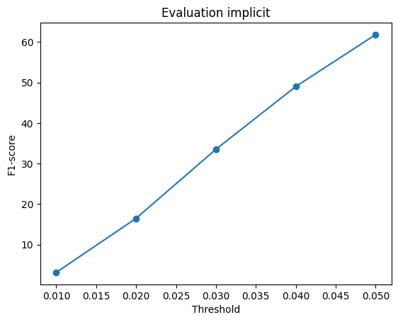
F1@0.05: 61.84
I query the occupancy at every point of a 32×32×32 grid in (-1, 1)3.
Each xyz coordinate is passed through a positional encoding (sin and cos at 6 frequencies). I took the idea of using frequency components of the input from NeRF.
The encoded point is concatenated with the 512-d ResNet18 image feature and passed through a 2-layer MLP (256 units, ReLU). The image feature is concatenated again before a second 2-layer MLP, which outputs one occupancy logit per point.
Loss: BCE with pos_weight 2, plus Dice. The mesh is extracted with marching cubes at 0.5.
The F1 score is lower than the voxel model's (61.84 vs. 73.19), and it does worse on thin parts such as the chair legs.
I trained it for only about 20 epochs, compared to about 100 for the voxel model. Training it longer would probably give better results.
Test example 0Test example 100Test example 400
F1 vs. threshold
3.2 Parametric network
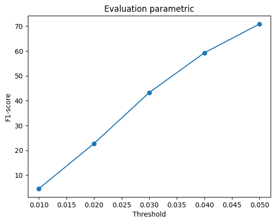
F1@0.05: 70.89
The model maps 2D points to 3D points, conditioned on the image.
It has 10 MLP heads. Each head takes 100 points sampled uniformly in [0, 1]2, concatenated with the 512-d image feature, and outputs their xyz positions (2 hidden layers of 256 units, LeakyReLU).
The outputs of the 10 heads are concatenated into a 1000-point cloud, trained with the chamfer loss.
The F1 score is lower than the voxel model's (70.89 vs. 73.19).
Visually, the results look better than the regular point cloud model's, but the outputs are very planar. The individual sheets from each MLP head are visible, and they do not always follow the surface of the object.
Adding more heads, so that each one covers a smaller part of the surface, would likely give better results.
Test example 100Test example 400Test example 500
F1 vs. threshold
3.3 Extended dataset for training
I trained the voxel model on chairs only and on chairs, cars and planes, with the same settings, and evaluated both on the 3-class test set.
Test class
Trained on chairs only
Trained on chair + car + plane
Chair (678)
73.30
70.13
Car (368)
53.67
76.56
Plane (405)
43.88
87.79
The car voxels in the extended dataset are stored with the x and z axes swapped compared to chairs and planes. With the provided evaluation, even the ground-truth car voxels only score about 50 F1. I therefore swapped the x and z axes when evaluating cars. Chairs and planes use the provided evaluation unchanged.
Each example shows the input image, the predictions of both models from that same image, and the ground truth.
Chair, test example 773Chair, test example 1111Chair, test example 1450Car, test example 405Car, test example 496Car, test example 680Plane, test example 0Plane, test example 101Plane, test example 303
On chairs, the model trained on all three classes has a slightly lower F1 score, but its predicted meshes look better than those of the chairs-only model.
I also ran the chairs-only model on cars and planes. As expected, it does not give coherent results for these objects, since it has never seen them during training.