Multi-view data preprocessing
20 pts


check_data.py (train, 4 samples)
| Sample | Valid depth | Max point reproj. (px) | Max ray reproj. (px) | Centroid dist. |
|---|---|---|---|---|
| e050c15a8d_frame_007080 | 0.978 | 1.1e-04 | 1.1e-04 | 1.0000 |
| 5f99900f09_frame_002820 | 0.990 | 1.2e-04 | 1.1e-04 | 1.0000 |
| 47b37eb6f9_frame_002720 | 0.961 | 9.9e-05 | 8.9e-05 | 1.0000 |
| 4c5c60fa76_frame_006690 | 0.752 | 1.2e-04 | 1.1e-04 | 1.0000 |
Batch shapes: rgb (2, 8, 3, 224, 224), depth (2, 8, 1, 224, 224), depth_valid (2, 8, 1, 224, 224), K (2, 8, 3, 3), frame_numbers (2, 8), T_world_from_camera (2, 8, 4, 4), original_world_from_reference (2, 4, 4), scene_scale (2,), points_world (2, 8, 3, 224, 224), ray_origins (2, 8, 3, 224, 224), ray_directions (2, 8, 3, 224, 224), plucker (2, 8, 6, 224, 224).
- Canonicalization
- Every pose is re-expressed relative to the first sampled camera, T′i = T0−1Ti, so camera 0 becomes the identity. Depth is unprojected in this frame, the distance s from the origin to the centroid of all valid points is computed, and translations, depth and points are divided by s. This removes the arbitrary world origin, orientation and metric scale of each scan, so every training sample has the same reference frame and roughly unit size.
- World-space ray directions
- For pixel (u, v), K−1[u, v, 1]T is the direction through that pixel centre in camera coordinates (z = 1). Rotating it by the camera-to-world rotation R (no translation: it is a direction) and normalizing gives the unit world direction d = R K−1[u, v, 1]T / ‖·‖; the ray origin is the camera centre t.
- Plücker moment
- m = o × d is perpendicular to the plane through the ray and the world origin, and with unit d its length is the distance from the origin to the ray. It does not change if o is replaced by any other point o + λd on the ray, so (d, m) identifies the line itself; d alone only gives the direction, m adds where the ray is. Since m scales with o, it is divided by the scene scale with the translations.
Mini-LVSM: overfitting
10 pts
Mini-LVSM: training and evaluation
30 ptsSettings: configs/lvsm.json trained for 400 epochs instead of
its 100 (validation PSNR was still rising at 100; that run is the baseline in 2.3). Patch
8, width 384, 8 layers, S = 2 sources and 6 targets per sample,
batch 4, AdamW lr 0.0002 with warm-up and cosine decay, bf16, 22,400 steps on one
GPU. Best checkpoint: epoch 387. Evaluation: the 28 validation scenes, 8 views from
the first 32 prepared frames.

| Source views S | Target rays | PSNR (dB) | SSIM |
|---|---|---|---|
| 1 | correct | 15.92 | 0.5890 |
| 1 | shuffled | 11.62 | 0.4804 |
| 1 | none | 12.46 | 0.5348 |
| 2 | correct | 17.23 | 0.6007 |
| 2 | shuffled | 11.24 | 0.4601 |
| 2 | none | 12.44 | 0.5317 |
| 4 | correct | 18.39 | 0.6227 |
| 4 | shuffled | 11.30 | 0.4579 |
| 4 | none | 12.44 | 0.5412 |
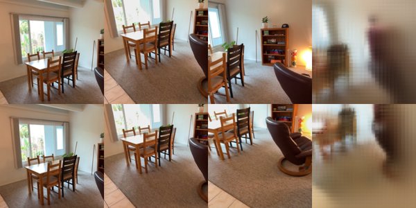


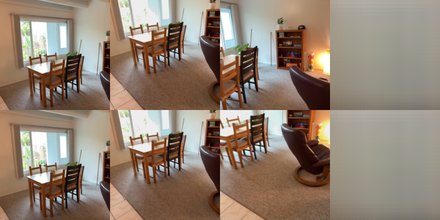
Each image: two of the target views (rows); columns are the S source views, the ground truth and the prediction.
- Number of source views
- More sources help at every metric. With one source, any part of the target outside or occluded in that view has to be guessed, and the depth of what is visible is ambiguous, so the model hedges with a blurry average; each extra source covers more of the target and adds parallax that fixes where content goes. Sources are random frames of a 32-frame window, so more sources also make it likelier that one is close to the target. The model was trained with S = 2 and still improves with 4, so it uses the extra context rather than overfitting to the training count.
- Target-ray conditioning
- The target rays are the only input that says which view to render. With zero rays every query token is identical up to its patch position, so the model outputs one nearly uniform image in the scene's mean colour and PSNR no longer depends on S. Shuffled rays are worse still: the model renders structure for a different viewpoint, and confidently wrong structure costs more MSE than a flat mean. Correct rays beat both by several dB, so the prediction really is driven by the target camera, not just by the source content.
Mini-LVSM: analysis and exploration
+10 bonusEvery run changes one thing from configs/lvsm.json and keeps its 100-epoch
schedule, so each is compared with that 100-epoch baseline, not with the Q2.2 model. Tables:
validation PSNR (dB) / SSIM with 1, 2 and 4 source views and correct target rays; one seed
per run.
Loss function
| Run | S = 1 | S = 2 | S = 4 |
|---|---|---|---|
| MSE (baseline) | 15.19 / 0.558 | 16.13 / 0.560 | 16.86 / 0.575 |
| MSE + L1 | 15.35 / 0.561 | 16.28 / 0.564 | 17.07 / 0.580 |
| MSE + 0.2 (1 − SSIM) | 14.78 / 0.576 | 15.43 / 0.580 | 15.81 / 0.594 |
| MSE + 0.5 perceptual | 13.60 / 0.550 | 13.78 / 0.549 | 13.90 / 0.560 |
| MSE + 0.02 perceptual | 15.02 / 0.563 | 15.87 / 0.562 | 16.42 / 0.574 |

Question: how do PSNR, SSIM and visual sharpness change when an L1, SSIM or perceptual term is added to the MSE? The perceptual term is the L1 distance between VGG-16 features (relu1_2 to relu4_3) of prediction and ground truth, tried at 0.5 and at 0.02.
Result: L1 gives a small gain in both PSNR and SSIM and slightly crisper edges: it penalizes small errors more than MSE does, so the model is pushed out of the blurry average sooner. The SSIM term trades PSNR for SSIM: it rewards local structure and contrast over absolute colour, and its predictions lose the patch-grid artefacts. The perceptual term at 0.5 collapses the output towards flat images. I checked why: on these blurry predictions the raw VGG-feature distance is far larger than the MSE, and it scores a flat mean-colour image as better than the baseline's blurry but correctly placed prediction, so it dominates training and pulls towards flatness. At 0.02 it trains normally but only adds a fine checkerboard texture (VGG artefacts), not real detail, and costs a little PSNR. None of the terms makes the predictions sharp: at this stage the blur comes from uncertainty about where content goes, which a different per-pixel or feature loss cannot resolve. Limitation: one weight per term (two for the perceptual one) and one seed.
Model capacity
| Run | S = 1 | S = 2 | S = 4 | Params (M) | Step (ms) | Mem (GB) | Render (ms) |
|---|---|---|---|---|---|---|---|
| p 8, D 384, 8 layers (baseline) | 15.19 / 0.558 | 16.13 / 0.560 | 16.86 / 0.575 | 14.6 | 236 | 9.0 | 76 |
| patch 16 | 15.02 / 0.551 | 15.87 / 0.552 | 16.47 / 0.564 | 16.0 | 55 | 2.6 | 17 |
| width 256 | 15.18 / 0.557 | 16.11 / 0.559 | 16.85 / 0.573 | 6.6 | 150 | 6.1 | 47 |
| width 512 | 15.17 / 0.557 | 16.13 / 0.560 | 16.77 / 0.575 | 25.8 | 332 | 12.0 | 107 |
| 4 layers | 15.09 / 0.555 | 15.98 / 0.557 | 16.59 / 0.571 | 7.5 | 122 | 4.8 | 39 |
| 12 layers | 15.21 / 0.559 | 16.17 / 0.561 | 16.86 / 0.576 | 21.7 | 355 | 13.2 | 114 |
Question: how do patch size, width and depth trade quality against cost? Step time and memory are for one training step (batch 4, 6 targets each) and render time for one forward pass, all timed back to back on one RTX A6000.
Result: width (256-512) and depth (4-12 layers) move PSNR by at most a few tenths of a dB: 4 layers is slightly worse and the larger models are no better, while time and memory grow roughly with the parameter count. No model reaches a higher PSNR on its training views than on validation, so at this schedule they are limited by optimization, not capacity, and extra parameters cannot help yet. Patch size is the knob that matters for cost: 16-px patches give 4× fewer tokens per view, so a training step is 4.3× faster and needs 3.4× less memory (attention runs over all (S+1)·N tokens), but quality drops because each token must decode a whole 16×16 patch from one vector, which makes the output blockier. Limitation: one seed and a short schedule; with longer training the larger models would likely pull ahead.
Training view count
| Run | S = 1 | S = 2 | S = 4 |
|---|---|---|---|
| train S = 1 | 15.12 / 0.559 | 14.91 / 0.552 | 14.65 / 0.561 |
| train S = 2 (baseline) | 15.19 / 0.558 | 16.13 / 0.560 | 16.86 / 0.575 |
| train S = 4 | 15.28 / 0.556 | 16.39 / 0.561 | 17.44 / 0.579 |
| train S ~ U{1..4} | 15.19 / 0.559 | 16.18 / 0.559 | 17.00 / 0.573 |
Question: does the number of source views used in training change how the model does with 1, 2 and 4 sources at test time? Runs train with S = 1, 2 (baseline), 4, or a new S drawn uniformly from 1-4 at every step; every sample still has 8 views, so fewer sources means more targets.
Result: training with S = 4 is best at every test S, including S = 1, probably because every step makes it fuse several views, which also teaches it to use a single view's content better. Training with S = 1 is the opposite: it never learns to combine sources, and more sources at test time make it worse, likely because the longer token sequence changes the attention statistics it was trained on. Random S matches the baseline at S = 1 and improves on it at S = 2 and 4, a middle ground that covers every count but sees many sources less often than the S = 4 run. Limitation: one seed; at a longer schedule the S = 4 run's lead at S = 1 may shrink.
Camera encoding
| Run | S = 1 | S = 2 | S = 4 |
|---|---|---|---|
| Plücker rays (baseline) | 15.19 / 0.558 | 16.13 / 0.560 | 16.86 / 0.575 |
| raw camera vector | 14.67 / 0.550 | 15.31 / 0.550 | 15.59 / 0.563 |
| Run | Target camera (S = 2) | PSNR (dB) |
|---|---|---|
| Plücker rays (baseline) | correct | 16.13 |
| Plücker rays (baseline) | shuffled | 11.48 |
| Plücker rays (baseline) | none | 12.43 |
| raw camera vector | correct | 15.31 |
| raw camera vector | shuffled | 11.67 |
| raw camera vector | none | 12.37 |

Question: do the per-pixel Plücker rays matter, or is the camera itself enough? In the raw variant each source token gets its RGB patch plus a projection of that view's 16-d camera vector (c2w [R | t], fx, fy, cx, cy normalized by image size), and each target query gets only the projected camera vector plus its patch position.
Result: Plücker rays are better at every S and the gap grows with S. With rays, every token already carries its own 3D ray, so matching a target patch to the source patches that see the same content is a comparison in one shared space. With one camera vector per view, the network first has to learn the pinhole projection (pose, intrinsics and patch position) inside attention, which it only partly manages at this schedule, so extra sources help it less. The raw model still uses its camera: shuffling or zeroing the target camera costs several dB. Limitation: one seed and a short schedule.
Mini-VGGT: overfitting
10 pts


Mini-VGGT: training and evaluation
30 ptsSettings: configs/vggt.json unchanged. Frozen DINOv2
dinov2_vitb14, 8 frame/global pairs of width 384 with 6 heads,
8 views from a 32-frame window, batch 16, AdamW (lr
0.0006, weight decay 0.01), 10 warm-up epochs then cosine
decay to 0.05×, loss = 5.0·camera + 1.0·depth, bf16,
1000 epochs on one GPU. best.pt is epoch 869 (lowest validation
loss). Evaluation: 8 views from the first 32 prepared frames, 224 px, seed 825.

| Metric | Validation (28 scenes) | Test (28 scenes) |
|---|---|---|
| Depth AbsRel ↓ | 0.143 | 0.156 |
| Depth δ1 ↑ | 0.819 | 0.807 |
| Rotation AUC @5 / 15 / 30° ↑ | 0.215 / 0.536 / 0.712 | 0.216 / 0.550 / 0.740 |
| Translation AUC @5 / 15 / 30° ↑ | 0.010 / 0.071 / 0.174 | 0.012 / 0.088 / 0.204 |
| Joint pose AUC @5 / 15 / 30° ↑ | 0.002 / 0.057 / 0.157 | 0.004 / 0.064 / 0.184 |


Errors on held-out scenes. Depth is the strongest part, rotation next, and translation the weakest. Within a 32-frame window the phone moves only a short distance, so the translation direction between two views is ill-conditioned: a small error in a predicted camera centre swings it by many degrees. That is why translation AUC at 5° is near zero while depth and rotation are good, and the joint pose AUC is held down by translation. In the viewers the layout of every room is recovered, but surfaces are thicker and noisier than the ground truth: depth bleeds across object boundaries (the head decodes 14-px patches with only a small RGB refinement), thin structures such as window frames and chair legs are smeared, and a view whose pose is slightly off adds a second, offset copy of a surface. Validation and test are close, and the validation camera loss flattens late in training while the training loss keeps falling, so what remains is mostly generalization from 224 training scenes rather than optimization.
Mini-VGGT: analysis and exploration
+10 bonusEach run changes one thing from configs/vggt.json and is trained for
300 epochs (Q3.2 uses 1000; at full length the six runs did
not fit my GPU budget), so every
comparison is against the 300-epoch baseline in the first row, not against Q3.2. All numbers:
validation split, Q3.2's evaluation protocol, one seed per run. Point errors are the mean
L2 distance to the GT point map over valid pixels, in normalized units.
| Run (300 epochs, val) | AbsRel ↓ | δ1 ↑ | Rot AUC@30 | Trans AUC@30 | Pose AUC@30 | Pts from depth+cam ↓ | Pts from head ↓ |
|---|---|---|---|---|---|---|---|
| Joint camera + depth (baseline) | 0.172 | 0.757 | 0.571 | 0.116 | 0.097 | 0.347 | – |
| + point-map head | 0.172 | 0.770 | 0.609 | 0.128 | 0.115 | 0.321 | 0.323 |
| Camera only | n/a | n/a | 0.593 | 0.135 | 0.117 | 0.771 | – |
| Depth only | 0.162 | 0.790 | n/a | n/a | n/a | 0.608 | – |
| Fine-tuned DINO | 0.158 | 0.802 | 0.555 | 0.123 | 0.105 | 0.326 | – |
| Trained with 4 views | 0.176 | 0.750 | 0.533 | 0.116 | 0.094 | 0.368 | – |
n/a: that head has zero loss weight in the run, so it is never trained; the points from depth + cameras still use it.
Point-map head vs. depth + cameras


Question: is a directly regressed point map better than unprojecting the predicted depth with the predicted cameras? I added a point head (same decoder as the depth head, 3 channels, no activation) trained with a trimmed L2 + gradient loss on the canonical GT points, weight 1, on top of the baseline losses.
Result: the two point clouds are about equally accurate (last two columns of the point-head row). They fail differently: depth + cameras keeps planar surfaces flat but smears points at depth edges and inherits every camera error as a rigid offset of that view; the point head has no such coupling and is smoother, but more diffuse. Adding the head also slightly improved depth δ1 and the camera AUCs of the shared trunk, which suggests the extra dense 3D supervision is a useful auxiliary signal. Limitation: one seed and a short schedule; differences this small are within what I would expect from seed noise.
Multi-task synergy
Question: does learning cameras and depth jointly help either task? Single-task runs set the other loss weight to 0, everything else unchanged.
Result: at this budget, no. Depth-only reaches a lower AbsRel and higher δ1 than the joint model, and camera-only reaches higher rotation and translation AUCs. With a shared 16-block trunk of width 384, the two losses compete for capacity, and nothing in the architecture forces depth and cameras to agree (each head is supervised separately), so neither task gets geometric information from the other. Joint training is still what gives a consistent reconstruction: only the joint model produces depth and cameras, so its unprojected point cloud is far better than either single-task model's. Adding the third (point) task, which does tie the two together in one 3D frame, was the one change that helped the camera metrics. Limitation: single seeds and small gaps; a longer schedule may change the balance.
Fine-tuning DINO
Question: does fine-tuning DINOv2 instead of freezing it improve the reconstruction? The encoder trains with the rest of the model at 0.05× the learning rate (so its pretrained features are adjusted, not overwritten), with gradient checkpointing on its 12 blocks: without it the 16 × 8-image batch ran out of memory on a 24 GB GPU.
Result: fine-tuning clearly helps depth (lower AbsRel, higher δ1) and with it the unprojected points, while the camera metrics are mixed: rotation AUC slightly lower, translation and pose AUC slightly higher. Frozen DINO features are built for semantic matching, which is already what relative pose needs; adapting them lets the dense head get finer local geometric cues (edges, surface orientation), which matter most for per-pixel depth. The cost is 1.3× the training time per epoch and the extra memory. Limitation: one learning-rate scale, one seed and a short schedule; with only 224 training scenes, a longer run risks overfitting the encoder.
Number of views
| Eval views | AbsRel (8-view train) | AbsRel (4-view train) | Rot AUC@30 (8) | Rot AUC@30 (4) | Trans AUC@30 (8) | Trans AUC@30 (4) | Forward (ms) | Peak mem (GB) |
|---|---|---|---|---|---|---|---|---|
| 2 | 0.127 | 0.130 | 0.570 | 0.564 | 0.126 | 0.121 | 30 | 0.69 |
| 4 | 0.158 | 0.160 | 0.561 | 0.514 | 0.140 | 0.126 | 31 | 0.71 |
| 8 | 0.172 | 0.176 | 0.571 | 0.533 | 0.116 | 0.116 | 38 | 0.75 |
| 16 | 0.220 | 0.217 | 0.523 | 0.486 | 0.111 | 0.111 | 48 | 0.83 |
| 32 | 0.221 | 0.216 | 0.520 | 0.486 | 0.103 | 0.105 | 99 | 0.98 |
Question: how does the number of input views change accuracy, runtime and memory,
at test time and in training? The baseline (trained with 8 views) and a copy trained with 4
views (configs/vggt_bonus/views4.json, otherwise identical) are each evaluated
with 2-32 views drawn from the first 32 frames of every validation sequence. Time and memory
are for one forward pass of one sequence, bf16, on an RTX A5000.
Result: camera accuracy is flat from 2 to 8 views and drops at 16 and 32, beyond the view count seen in training. Training with 4 views gives lower rotation AUC at every view count, including 4 (translation AUC is about the same): an 8-view sample supervises 28 relative poses instead of 6 and gives global attention more cross-view context to learn from. Depth AbsRel grows with the number of views for both models alike, so it is not a training effect. Frame 0 is always included and the scale is the centroid distance of all selected views' points, so with more views, spread over 32 frames, the normalized depth of each view depends on scene content it cannot see, which is harder to predict. Runtime is nearly flat up to 8 views, where the per-view DINO and frame attention dominate, then grows quickly because global attention is quadratic in V × 261 tokens; memory grows only slowly at batch 1, since attention is computed without storing the attention matrix. Limitation: one seed; more views also means frames further from the reference.