Ray sampling
5 pts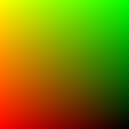
xy_grid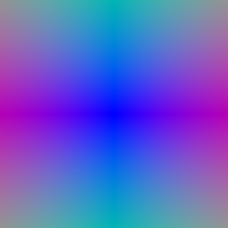
Point sampling
5 pts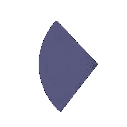
Volume rendering
20 pts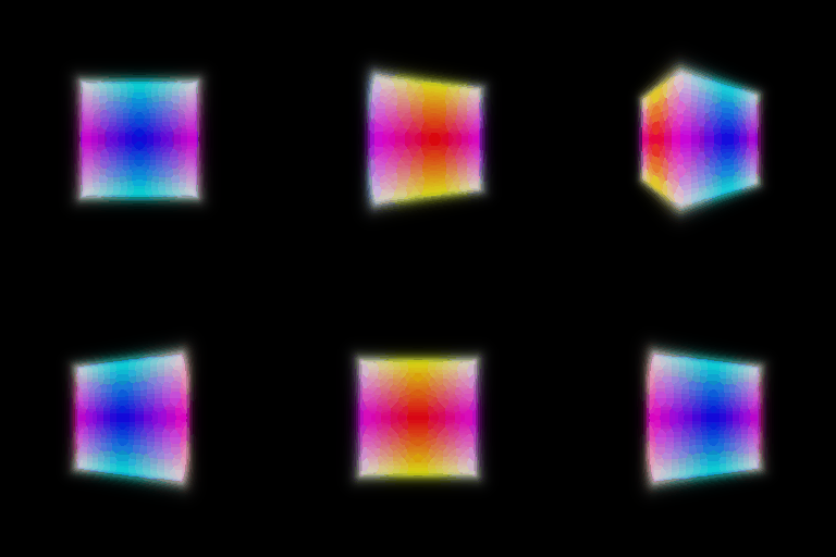
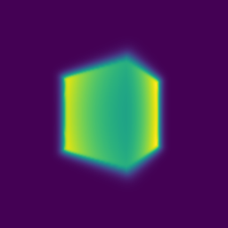
Optimising a basic implicit volume
10 pts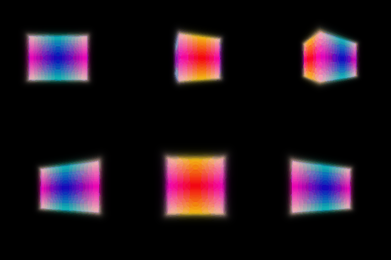
Neural Radiance Field
20 pts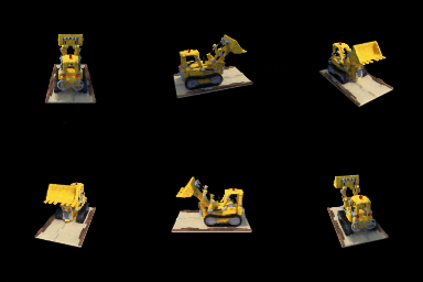
nerf_lego.yaml).The MLP maps the harmonic embedding of a point (6 frequencies) through 6 ReLU layers of width 128, with the embedding re-injected at layer 3; a ReLU head gives density and a small sigmoid head gives colour. No view dependence.
View dependence
+10 EC| Materials, 128×128 | Train PSNR (10 views) | Held-out PSNR (100 views) |
|---|---|---|
| No view dependence | 22.54 | 23.31 |
| View dependent, Ldir = 2 | 23.36 | 24.02 |
| View dependent, Ldir = 6 | 23.31 | 23.95 |
Same network and schedule (nerf_materials.yaml, 250 epochs) in all three runs.
View dependence: the direction's harmonic embedding (Ldir frequencies) is
concatenated to the position feature after the density head, so density stays a function of
position only and just the colour head sees the direction.

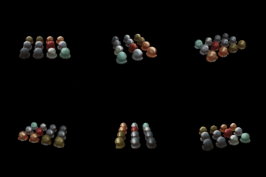


nerf_materials_highres.yaml), held-out PSNR 24.33.Trade-off. Letting colour depend on direction lets the model reproduce the specular highlights of the metallic spheres; without it, a highlight that moves with the camera can only be averaged into a fixed, duller colour, so the no-view-dependence model is flatter and scores 0.7 dB lower on held-out views. But more direction capacity is not better: with Ldir = 6 the colour can change quickly with angle, and since each surface point is seen from only ~100 training directions, it starts fitting per-view detail that does not transfer. Its highlights are grainier and its held-out PSNR is lower than with Ldir = 2 (23.95 vs 24.02). Feeding the direction only into the colour head, through a low-frequency embedding, is what keeps view dependence from overfitting: geometry must still explain all views at once.
Coarse/fine sampling
+10 EC| Lego, 128×128, 250 epochs | Network evals / ray | Held-out PSNR | Train s / epoch | Render s / image |
|---|---|---|---|---|
| Single network, 128 samples | 128 | 23.70 | 2.2 | 0.15 |
| Single network, 256 samples | 256 | 23.98 | 3.9 | 0.28 |
| Coarse/fine (64 + 128 samples) | 64 + 192 | 24.18 | 4.0 | 0.28 |
Coarse/fine: a coarse NeRF is evaluated at 64 stratified samples; its weights define a piecewise-constant pdf along the ray, from which 128 more depths are drawn by inverse-transform sampling; the fine NeRF (same architecture) is evaluated at all 192 sorted depths and gives the output. Both networks are trained with the photometric loss. All three runs use the same schedule and were trained back to back on the same GPU; held-out PSNR is over the 100 validation views.


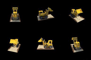
Speed vs quality. Coarse/fine gives the best held-out PSNR, 0.5 dB above the single 128-sample network, but costs 1.9× the training time per epoch and 1.9× the render time, because every ray now runs 256 network evaluations instead of 128. Spending the same budget on uniform samples (single network, 256 samples) recovers only part of that gain (0.3 dB): coarse/fine puts its extra samples near the surfaces, where the weights are concentrated, instead of in empty space, so at equal cost it is still 0.2 dB better. Visually the difference is small at 128×128; edges of the tracks and bucket are slightly crisper.
VolSDF
10 pts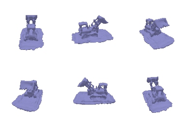
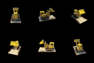
α and β. Density is σ(x) = α Ψβ(−d(x)), where Ψβ is the CDF of a zero-mean Laplace distribution with scale β. α is the density deep inside the object: how opaque the solid is. β is the width of the transition: density rises from 0 to α over a band of a few β around the zero level set, and as β → 0 it becomes α times the indicator of the inside.
Effect of β (everything else fixed)



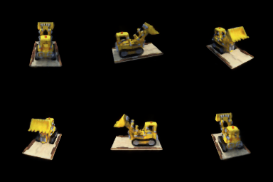
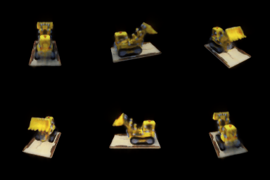
- 1. How does high / low β bias the learned SDF?
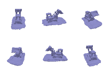
- High β spreads density over a thick band around the surface, so the rendered object is a soft shell and the SDF that explains the images is smoothed and inflated: at β = 0.2 the base becomes a thick rounded slab and fine parts lose detail. Low β makes density nearly a step at the zero level set, so the SDF is pushed to the exact boundary, but only points very close to the surface receive any signal.
- 2. Easier to train with low or high β?
- High β. A wide transition gives non-zero density, and so gradient, to many samples along each ray even when the current surface is far from the true one. With low β the gradient lives in a thin band that the fixed 128 samples per ray can miss, which makes optimisation less stable (the β = 0.02 run has a dark floater streak in its colour render).
- 3. More accurate surface with low or high β?
- Low β. The rendering weight then peaks sharply at the zero level set, so the colour loss pins the surface in place rather than a blurry shell around it; the β = 0.02 and 0.05 surfaces are visibly sharper than the 0.2 one.
Settings. The best result (top) uses the provided volsdf_surface.yaml:
α = 10, β = 0.05, eikonal weight 0.02, 250 epochs. The distance MLP
(6 layers, width 128) uses Softplus(100) activations and is initialised to the SDF of a sphere,
so the eikonal term holds from the start and there is a well-defined surface from the first
epoch. β = 0.05 sits between the two failure modes above: almost as sharp as 0.02,
without its floaters.
3D Gaussian rasterization
35 pts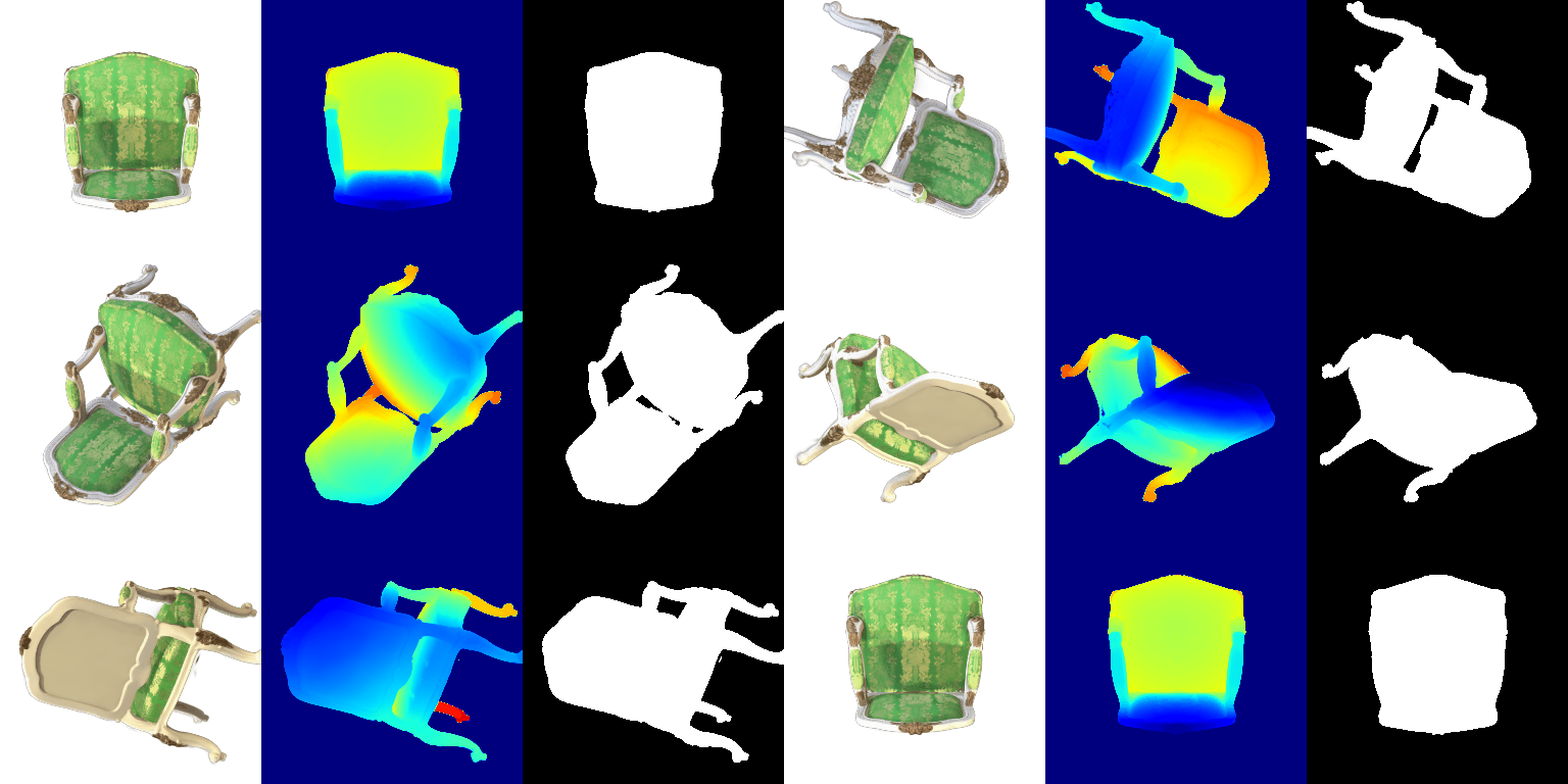
render.py.Training 3D Gaussians
15 pts| Parameter | Adam learning rate |
|---|---|
| means | 0.0005 |
| scales | 0.005 |
| colours | 0.02 |
| opacities | 0.05 |
Isotropic Gaussians initialised from the provided point cloud, L1 loss, Adam. PSNR and SSIM are the means over the held-out views.
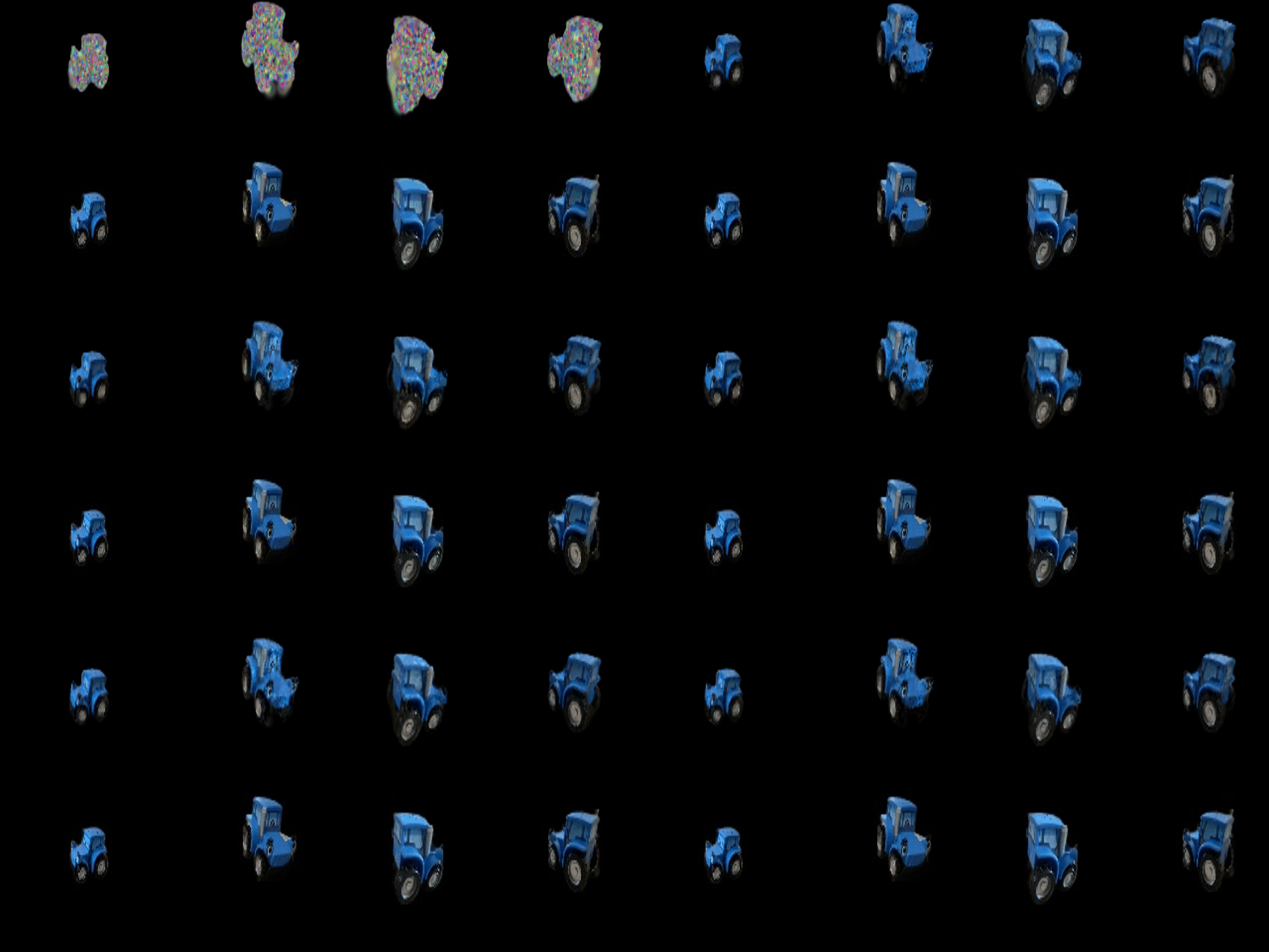
part_6_training_progress.gif: renders of four training views (top) against the ground truth (bottom) over the 3,000 iterations.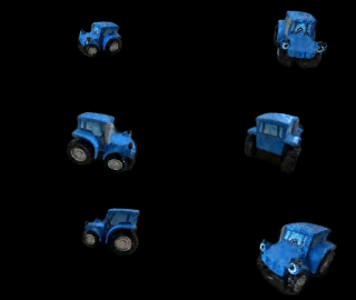
part_6_training_final_renders.gif: every training view after training.Rendering with spherical harmonics
10 pts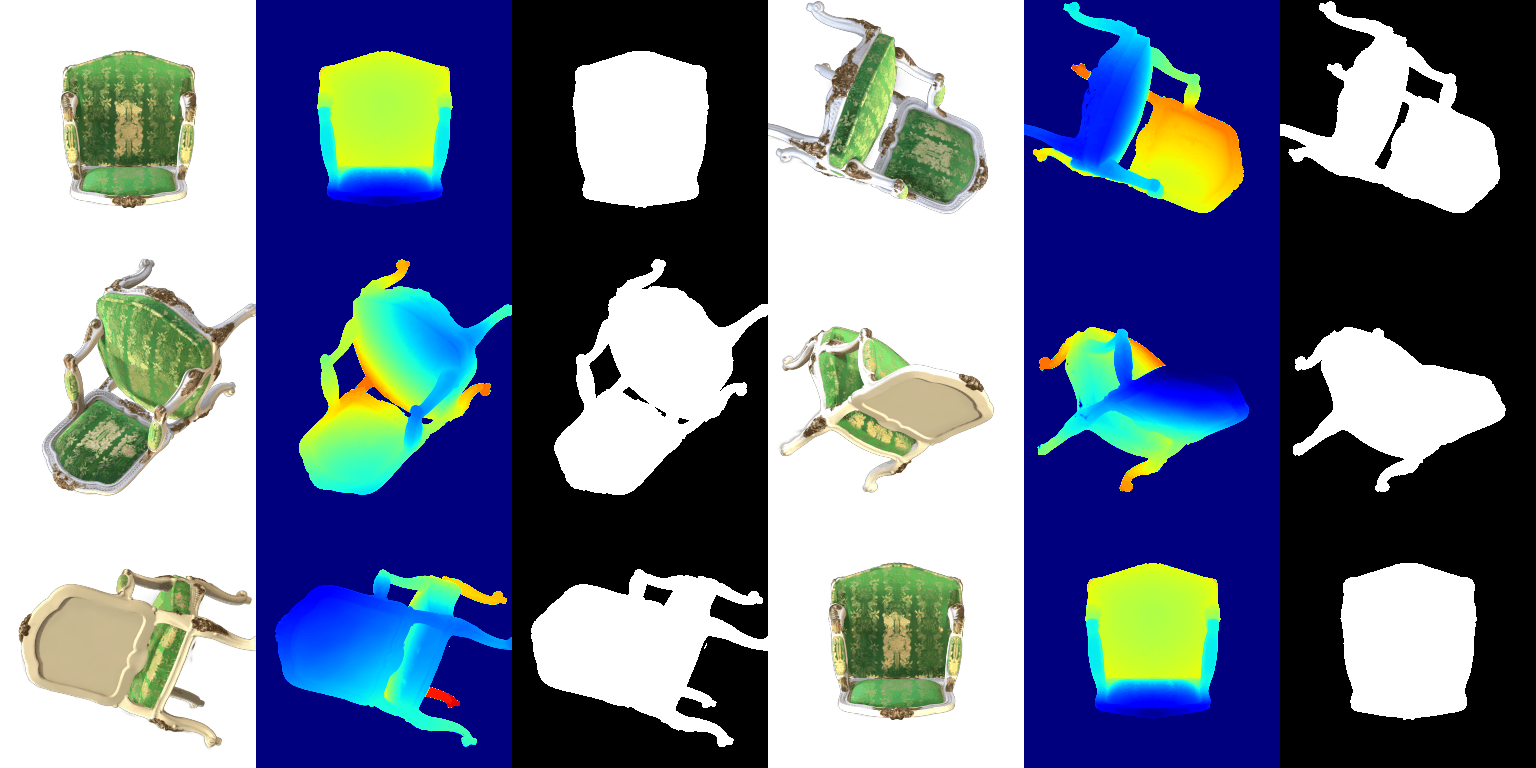
Front view (frame 0)

With SH the backrest is a darker, more saturated green and the gold brocade stands out much more; the DC-only version is flatter and lighter, because the DC term is the colour averaged over all view directions, so view-dependent sheen gets baked in as a uniform wash.
Top-down view (frame 8)

The same on the seat: SH recovers the dark-green/gold contrast of the fabric, and the side of the backrest cushion catches a highlight that the DC rendering does not have. The white frame looks almost the same in both.
Underside (frame 24)
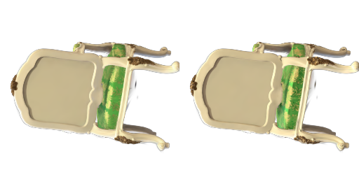
Almost no difference. The underside is a plain, matte, uniformly coloured surface with little view-dependent appearance, so its higher-order coefficients contribute little and the DC colour already explains it.
Training on a harder scene
+10 EC| Run (each adds to the one above) | PSNR | SSIM | Gaussians |
|---|---|---|---|
| Baseline (Q6 setup) | 18.41 | 0.705 | 10,000 |
| + wider random init | 22.74 | 0.832 | 10,000 |
| + anisotropic, SSIM loss, means lr decay | 23.22 | 0.860 | 10,000 |
| + densification (improved) | 23.64 | 0.874 | 17,060 |
Materials at 128×128 from 10,000 randomly initialised Gaussians, 3,000 iterations in every
run; PSNR / SSIM are means over the 100 validation views. The baseline is exactly the Q6 setup
(isotropic, the Q6 learning rates, L1 loss, default init_type="random"); each row
below it adds one change to the row above.
Best run: learning rates
| Parameter | Adam learning rate |
|---|---|
| means | 0.0005 → 5e-06 (exponential decay) |
| scales | 0.005 |
| colours | 0.02 |
| opacities | 0.05 |
| quaternions | 0.001 |
- Wider random initialisation
- The default draws means from N(0, 0.2²), a small blob at the centre, while the objects extend ~1.3 units from it; Gaussians far from an object get almost no gradient, so the outer spheres are never reached (blurry ghosts in the baseline). Drawing means from N(0, 0.6²) with an initial scale of 0.02 puts Gaussians near every object from the start. This is the largest single gain.
- Anisotropic Gaussians, SSIM loss, decaying means learning rate
- Rotations and three scales per Gaussian are trained (quaternion lr 1e-3), so one Gaussian can cover an elongated or curved patch; the loss is 0.8 L1 + 0.2 (1 − SSIM) as in the 3DGS paper, which rewards local structure and contrast rather than only per-pixel colour; the means learning rate decays exponentially from 5e-4 to 5e-6, so positions settle instead of jittering late in training.
- Simplified adaptive density control
- Every 250 iterations (750, 1,000, …, 2,750), the 10% of Gaussians with the largest average positional gradient (regions the current Gaussians cannot fit) are each split into two Gaussians 1.6× smaller, sampled inside the parent, and Gaussians with opacity below 0.005 are pruned (cap 30,000). The optimizer is rebuilt after each step.
Baseline (Q6 setup): training progress
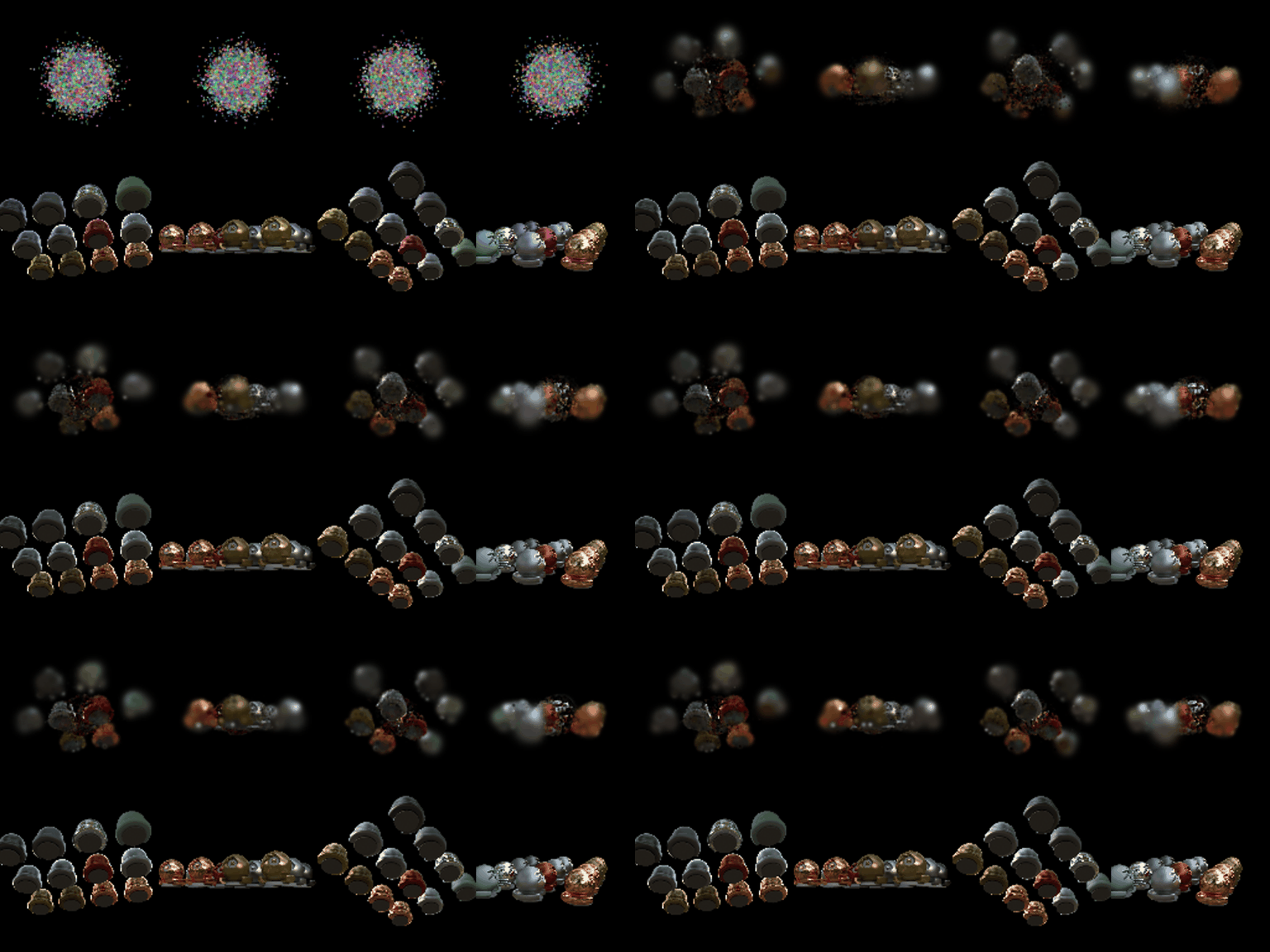
+ densification (improved): training progress
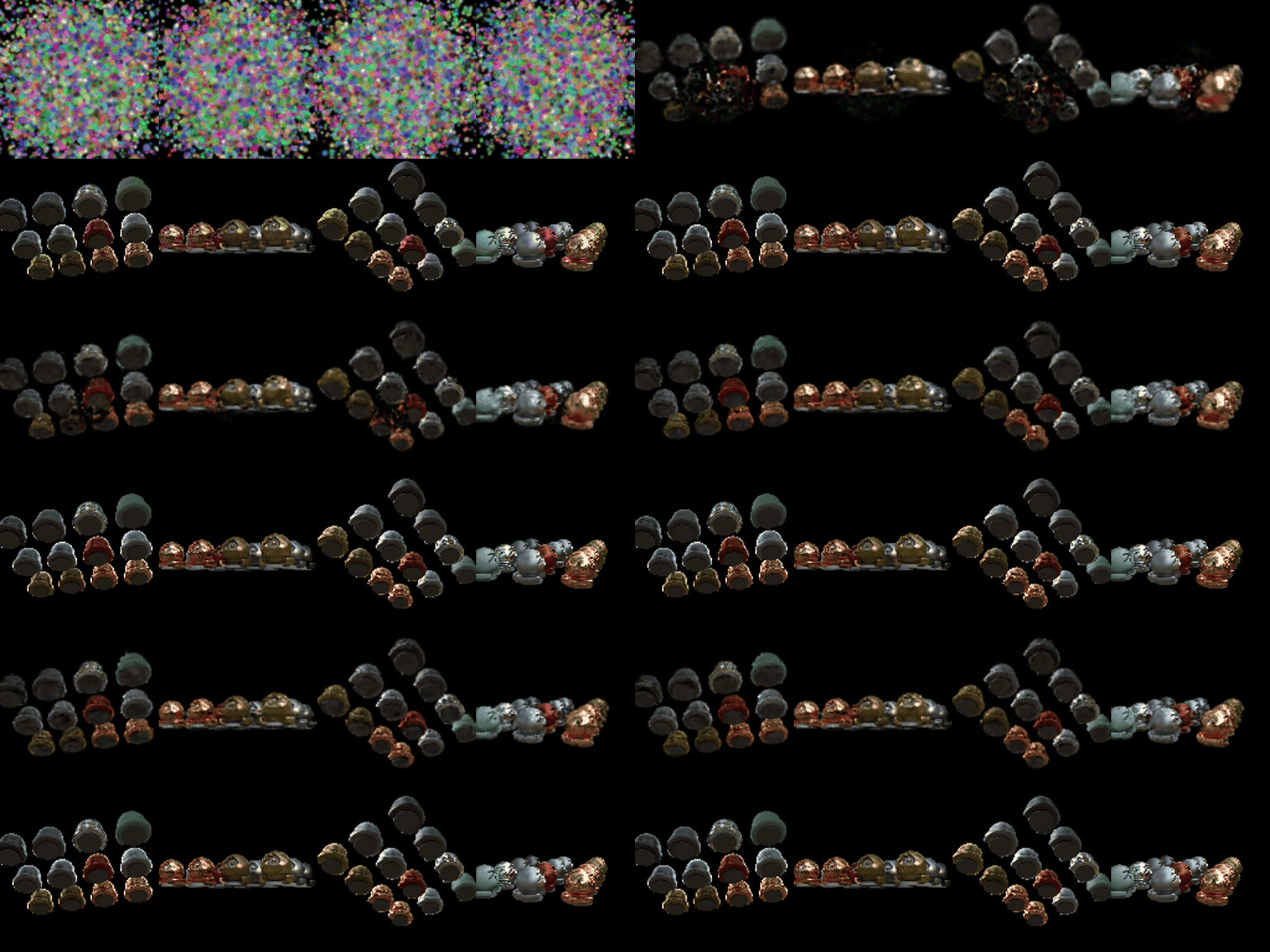
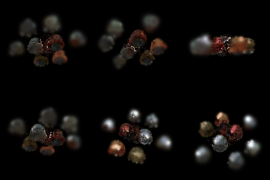
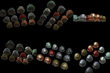
Comparison. The baseline never recovers the objects at the edge of the scene, and those it does are blurry; the improved run reproduces all objects with sharp outlines and shading. It also converges much faster: by iteration ~500 every object is already in place, while the baseline is still a central cluster with blurry blobs at the edges. The colour is still view-independent, so moving highlights are averaged into each Gaussian's colour.